Week 3 - Taylor table method and Matlab code

Aim: Deriving 4th order approximations of the second-order derivative. using central difference, skewed right-sided difference, skewed left-sided difference.

Second Order derivative of fourth order approximation,the method we will be using here is taylor’s table method

Second order derivative is given as:

Ә²Y/Әx²

If we consider a ordinary differential equation assume

Y = sin(x)/x²

So we can calculate second order differential just by differentiating it twice well but for complex problem we need lot of time and effort to solve such problems and get results So in such situation we can use taylor table method.

Before understanding taylor table method let us recap a basics of different schemes used for approximation such as:

• Forward differencing scheme
• Backward differencing scheme
• Central differencing scheme

Forward difference approximation:

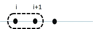
In this technique we choose definite function at point (i) and forward point (i+1) and the boundary is known as stencil. This is generally first order equation.

equation1 = (f(x+dx)-f(x))/dx

Backward difference approximation:

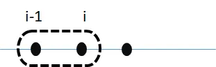
In this technique we choose definite function at point (i) and backward point (i-1) and the boundary is known as stencil. This is generally first order equation.

equation2 = (f(x)-f(x-dx))/dx

Central difference approximation:

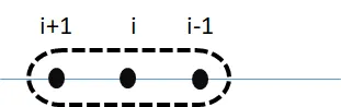
In this technique we choose definite function at point (i) and points both from backward (i-1) and forward (i+1) from the function the boundary is known as stencil, this is generally second order equation.

equation3 = (f(x+dx)-f(x-dx))/(2*dx)

We will use above methods but in form of skewed right side difference, skewed left side difference and central difference to derive second Order derivative of fourth order approximation.

Calculation of equation for any single node in stencil:

f(i+2) = f(i) + 2∆x f’(i) + ((2∆x)2/2!) f’’(i)+ ((2∆x)3/3!) f’’’(i)+ ((2∆x)4/4!) f’’’’ (i)+ ((2∆x)5/5!) f’’’’’(i)

We can derive any point with same logic as above and fill taylor table.

Taylor table for all the equations till 4th order/Universal taylor table:

stencil	f(i)	∆X f’(i)	∆X f’’(i)	∆X f’’’(i)	∆X f’’’’(i)	∆X f’’’’’(i)
f(i-5)	1	-5	25/2	-125/6	1024/24	-3125/120
f(i-4)	1	-4	8	-32/3	256/24	-1024/120
f(i-3)	1	-3	9/2	-9/2	81/24	-243/120
f(i-2)	1	-2	2	-4/3	2/3	-32/120
f(i-1)	1	-1	1/2	-1/6	1/24	-1/120
f(i)	1	0	0	0	0	0
f(i+1)	1	1	1/2	1/6	1/24	1/120
f(i+2)	1	2	2	4/3	2/3	32/120
f(i+3)	1	3	9/2	9/2	81/24	243/120
f(i+4)	1	4	8	32/3	256/24	1024/120
f(i+5)	1	5	25/2	125/6	1024/24	3125/120

We will use this taylor table for deriving different schemes.

Skewed Right side difference:

It uses a central difference scheme but nodes to be considered are right hand side values/positive values.

Number of nodes in the stencil N =The order of accuracy P+ order of derivative Q (one-sided/skewed schemes)

N=4+2=6(no of nodes)

skewed right side approximation:

(∂2y/dx2) = ( f(i)+f(i+1)+f(i+2)+f(i+3)+f(i+4)+f(i+5))/ ∆x2

Taylor table:

A*f(i)	1	0	0	0	0	0
B*f(i+1)	1	1	1/2	1/6	1/24	1/120
C*f(i+2)	1	2	2	4/3	2/3	32/120
D*f(i+3)	1	3	9/2	9/2	81/24	243/120
E*f(i+4)	1	4	8	32/3	256/24	1024/120
G*f(i+5)	1	5	25/2	125/6	1024/24	3125/120

Equations:

A+B+C+D+E+G=0

B+2C+3D+4E+5G=0

(1/2)B+2C+(9/2)D+8E+(25/2)G=1

(1/6)B+(4/3)C+(9/2)D+(32/3)E+(125/6)G=0

(1/24)B+(2/3)C+(81/24)D+(256/24)E+(1024/24)G=0

(1/120)B+(32/120)C+(243/120)D+(1024/120)E+(3125/120)G=0

We have six unknowns with six equation hence we can calculate co-efficients using matix.

Skewed left side difference:

It uses a central difference scheme but nodes to be considered are left hand side values/negative values.

Number of nodes in the stencil N =The order of accuracy P+ order of derivative Q

N=4+2=6(no of nodes)

(∂2y/dx2) = ( A*f(i)+B*f(i-1)+C*f(i-2)+D*f(i-3)+E*f(i-4)+G*f(i-5))/ ∆x2

Taylor table:

stencil	f(i)	∆X f’(i)	∆X f’’(i)	∆X f’’’(i)	∆X f’’’’(i)	∆X f’’’’’(i)
A*f(i-5)	1	-5	25/2	-125/6	1024/24	-3125/120
B*f(i-4)	1	-4	8	-32/3	256/24	-1024/120
C*f(i-3)	1	-3	9/2	-9/2	81/24	-243/120
D*f(i-2)	1	-2	2	-4/3	2/3	-32/120
E*f(i-1)	1	-1	1/2	-1/6	1/24	-1/120
G*f(i)	1	0	0	0	0	0

Equations:

A+B+C+D+E+G=0

-B-2C-3D-4E-5G=0

(1/2)B+2C+(9/2)D+8E+(25/2)G=0

-(1/6)B-(4/3)C-(9/2)D-(32/3)E-(125/6)G=0

(1/24)B+(2/3)C+(81/24)D+(256/24)E+(1024/24)G=0

-(1/120)B-(32/120)C-(243/120)D-(1024/120)E-(3125/120)G=0

Central difference:

It is same as central difference scheme.

No of nodes required for fourth order approximation, 2nd order derivative is:

Number of nodes in the stencil N =The order of accuracy P+ order of derivative Q -1 (symmetric/central schemes)

N=4+2-1

N=5(number of nodes)

(∂2y/dx2) = ( f(i-2)+f(i-1)+f(i)+f(i+1)+f(i+2))/ ∆x2

Taylor table:

f(i-2)	1	-2	2	-4/3	2/3
f(i-1)	1	-1	1/2	-1/6	1/24
f(i)	1	0	0	0	0
f(i+1)	1	1	1/2	1/6	1/24
f(i+2)	1	2	2	4/3	2/3

We can formulate equation for this scheme to and get values of co-efficients using matrix.

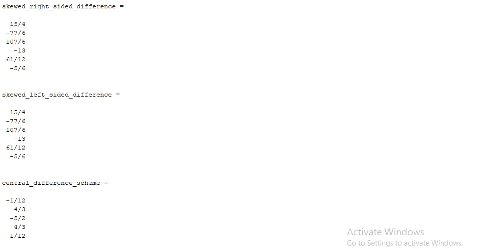
Values of co-efficient for all schemes:

Matlab program for calculation of co-efficients for all schemes:

close all
clear all
clc
%finding value of co-efficients for skew right-sided difference
A1 = [1 1 1 1 1 1;0 1 2 3 4 5;0 1/2 2 9/2 8 25/2;0 1/6 4/3 9/2 32/3 125/6;0 1/24 16/24 81/24 256/24 625/24;0 1/120 32/120 243/120 1024/120 3125/120]
C1 = [0;0;1;0;0;0];
right_sided_difference = inv(A1)*C1; 
coeff1 = sym(right_sided_difference) %convert decimal value to fraction
%finding value of co-efficients for skew left-sided difference
A2 = [1 1 1 1 1 1;0 -1 -2 -3 -4 -5;0 1/2 2 9/2 8 25/2;0 -1/6 -4/3 -9/2 -32/3 -125/6;0 1/24 16/24 81/24 256/24 625/24;0 -1/120 -32/120 -243/120 -1024/120 -3125/120]
C2 = [0;0;1;0;0;0];
left_sided_difference = inv(A2)*C2; 
coeff2 = sym(left_sided_difference)
%finding value of co-efficients for central difference
A3 = [1 1 1 1 1 ;-2 -1 0 1 2 ;2 1/2 0 1/2 2 ;-8/6 -1/6 0 1/6 8/6;16/24 1/24 0 1/24 16/24]
C3 = [0;0;1;0;0];
central_difference = inv(A3)*C3
coeff3 = sym(central_difference)

Matlab program for calculating and plotting all the schemes:

clear all
close all
clc
x = pi/3;
analytic_solution= -2*exp(x)*sin(x);
dx= linspace(pi/400,pi/40,20); %array of dx
 
%loop for range of dx
for i=1:length(dx)
    skewed_right_side_solution(i) = skewed_right_side(x,dx(i));
    skewed_left_side_solution(i) = skewed_left_side(x,dx(i));
    central_difference_solution(i) = central_difference(x,dx(i));
end

%plotting
figure(1)
loglog(dx,skewed_right_side_solution,'b')
hold on
loglog(dx,skewed_left_side_solution,'m--')
loglog(dx,central_difference_solution,'g')
legend({'skewed right side approx','skewed left side spprox','central difference'},'Location','northwest')
xlabel('dx values')
ylabel('error')

Function for calculation of skewed right side error:

function [skewed_right_side_error]= skewed_right_side(x,dx)
analytic_solution= -2*exp(x)*sin(x);
a=15/4;
b=-(77/6);
c=107/6;
d=-13;
e=61/12;
g=-(5/6);
skewed_right_side_approx= ((((a*(exp(x).*cos(x)))+(b*(exp(x+dx).*cos(x+dx)))+(c*(exp(x+2*(dx)).*cos(x+2*(dx))))+(d*(exp(x+3*(dx)).*cos(x+3*(dx))))+(e*(exp(x+4*(dx)).*cos(x+4*(dx))))+(g*(exp(x+5*(dx)).*cos(x+5*(dx))))))/(dx.^2));
skewed_right_side_error= abs(analytic_solution - skewed_right_side_approx);
end

Function for calculation of skewed left side error:

function [skewed_left_side_error]= skewed_left_side(x,dx)
analytic_solution= -2*exp(x)*sin(x);
a=15/4;
b=-(77/6);
c=107/6;
d=-13;
e=61/12;
g=-(5/6);
skewed_left_side_approx= ((((a*(exp(x)).*cos(x)))+(b*(exp(x-(dx)).*cos(x-(dx))))+(c*(exp(x-2*(dx)).*cos(x-2*(dx))))+(d*(exp(x-3*(dx)).*cos(x-3*(dx))))+(e*(exp(x-4*(dx)).*cos(x-4*(dx))))+(g*(exp(x-5*(dx)).*cos(x-5*(dx)))))/(dx.^2))
skewed_left_side_error= abs(analytic_solution - skewed_left_side_approx);
end

Function for calculation of central difference error:

function [central_difference_error]= central_difference(x,dx)
analytic_solution= -2*exp(x)*sin(x);
a= -1/12;
b=  4/3;
c=  -5/2;
d=   4/3;
e= -1/12;
central_difference_approx =((((a*(exp(x-2*(dx)).*cos(x-2*(dx))))+(b*(exp(x-dx).*cos(x-dx)))+(c*(exp(x).*cos(x)))+(d*(exp(x+(dx)).*cos(x+(dx))))+(e*(exp(x+2*(dx)).*cos(x+2*(dx))))))/(dx.^2));
central_difference_error= abs(analytic_solution - central_difference_approx);
end

Plot:

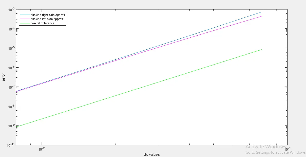
This plot explains the value of absolute error from all the schemes VS range of dx.

For fourth order central differencing scheme the values of error is least then skewed right and left sided scheme.

In this equation central difference scheme is more stable and skewed right side scheme is least.

But in case if we want to include boundary in our problem skewed scheme is more preferred.