Week 5 - Mid term project - Solving the steady and unsteady 2D heat conduction problem
Aim: Deriving 2D heat conduction equation for steady, unsteady, implicit, and explicit conditions, Using different iterative techniques such as jacobi, gauss siedel, and successive over relaxation.
Introduction:
To use navier stokes equation, we should rather divide a equation in several parts, and learn to solve each part which will make us familiar with all the optimization techniques used to get best solution.
In this challenge we will be solving second order derivative and time derivative, the equation which is also been known as 2-dimensional heat conduction equation.
In this derivation we will learn how the temperture varies in material, also the time and number of iteration it will take to reach steady state.
The different states in which we will be calculating above equation are:
- Steady state(Explicit)
- Unsteady state(Explicit)
- Unsteady state(Implicit)
The different iterative methods used to solve equation are:
- Jacobi method
- Gauss siedel method
- Successive over relaxation and successive under relaxation
Steady state(explicit):
3-dimensional transient/Unsteady heat conduction equation:
(∂T/∂t)= α( (∂2T/∂x2)+(∂2T/∂y2)+(∂2T/∂z2))
In this challenge we will be solving 2-dimensional heat conduction hence equation changes to:
(∂T/∂t)= α( (∂2T/∂x2)+(∂2T/∂y2))
(∂T/∂t)= α (∇2T)
For steady state heat conduction:
(∇2T)= 0
When we have time derivative in our equation according to method of charateristics we should use time marching to get a solution, In transient state heat conduction we have time derivative so we will solve this equation using time marching.
(∂T/∂t)= α (∇2T)
LHS = (Tn+1(i,j) - Tn(i,j) )/ ∆t
RHS = α*((T(i+1,j) - 2 T(i,j) + T(i-1,j) )n/ ∆X2 ) + ((T(i,j+1) - 2 T(i,j) + T(i,j-1) )n/ ∆Y2))
Where,
T(i+1,j) = TR = Right side boundary temperature
T(i,j) = TP = center boundary temperature
T(i-1,j) = TL = left side boundary temperature
T(i,j+1) = TT = top side boundary temperature
T(i,j-1) = TB = bottom side boundary temperature
((Tn+1P - Tnp)/ ∆t) = α*((TR - 2 TP + TL )n/ ∆X2 ) + ((TT - 2 TP + TB )n/ ∆Y2))
K1 = α*(∆t/∆X2)
K2 = α*(∆t/∆Y2)
Tn+1P = Tnp + K1*(TR - 2 TP + TL )n + K2*(TT - 2 TP + TB )n
This is a general equation for transient state explicit method, In which the right side of the equation is at time step 'n' which are known, hence we can calculate the temperature values for intermediate nodes easily.
In case of implicit method the values on RHS are unknown's hence equation changes to:
Tn+1P = (Tnp + K1*(TR + TL )n+1 + K2*(TT + TB )n+1 )/(1+2*K1+2*K2)
Steady state heat conduction:
(∂2T/∂x2)+(∂2T/∂y2) = 0
(TR - 2 TP + TL )n/ ∆X2 ) + ((TT - 2 TP + TB )n/ ∆Y2) = 0
(TR + TL )n/ ∆X2 ) + ((TT + TB )n/ ∆Y2) = k*TP
Where,
K=(2*(∆X2 + ∆Y2)/( ∆X2 *∆Y2))
Iterative methods:
In computational mathematics, an iterative method is a methematical procedure that uses an initial value to generate a sequence of improving approximate solutions for a class of problems, in which the n-th approximation is derived from the previous ones.
A specific implementation of an iterative method, including the termination criteria, is an algorithm of the iterative method.
An iterative method is called convergent if the corresponding sequence converges for given initial approximations.
In contrast, direct methods attempt to solve the problem by a finite sequence of operations. In the absence of rounding error, direct methods would deliver an exact solution (like solving a linear system of equations Ax=b by Gauss elimination).
Iterative methods are often the only choice for nonlinear equation(the equation whose output is not proportional to change in input). However, iterative methods are often useful even for linear problems involving many variables (sometimes of the order of millions), where direct methods would be prohibitively expensive (and in some cases impossible) even with the best available computing power.
Steady state equation for jacobi, gauss siedel and successive over relaxation for 2-D heat conduction:
Jacobi method:
TP = ((ToldR + ToldL )n/ ∆X2 ) + ((ToldT + ToldB )n/ ∆Y2)) /k
In jacobi method we assign boundary condition and form a matrix which is assigned to variable Told and use this value for calculation of 1st iteration.
Gauss siedel method:
TP = ((TR + ToldL )n/ ∆X2 ) + ((TT + ToldB )n/ ∆Y2)) /k
In gauss siedel for 1st iteration we use value calculated previously which are known such as at node 'n-1'.
Successive over relaxation:
TP = (1-W)*TnP + W*(((TR + ToldL )n/ ∆X2 ) + ((TT + ToldB )n/ ∆Y2)) /k)
In successive over relaxation method we add a relaxation factor to increase the weightage of gauss siedel/jacobi method which will decrease a no of iteration if the value of W>1 and sometime when we don't get answer using any of methods then SOR can be used to get solution.
Transient state equation for jacobi, gauss siedel and successive over relaxation for 2-D heat conduction(Explicit method):
jacobi method
Tn+1P = Tnp + K1*(TR - 2*ToldP + ToldL )n + K2*(TT - 2*ToldP + ToldB )n
Gauss siedel method:
Tn+1P = Tnp + K1*(TR - 2*ToldP + ToldL )n + K2*(TT - 2*ToldP + ToldB )n
Successive over relaxation:
Tn+1P =(1-W)*Tnp + W*(Tnp + K1*(TR - 2*ToldP + ToldL )n + K2*(TT - 2*ToldP + ToldB )n)
Transient state equation for jacobi, gauss siedel and successive over relaxation for 2-D heat conduction(Implicit method):
jacobi method
Tn+1P = (Tnp + K1*(ToldR + ToldL )n+1 + K2*(ToldT + ToldB )n+1 )/(1+2*K1+2*K2)
Gauss siedel method:
Tn+1P = (Tnp + K1*(TR + ToldL )n+1 + K2*(TT + ToldB )n+1 )/(1+2*K1+2*K2)
Successive over relaxation:
Tn+1P =(1-W)*Tnp + W*((Tnp + K1*(TR + ToldL )n+1 + K2*(TT + ToldB )n+1 )/(1+2*K1+2*K2))
Steps/logic:
- Define the values of inputs.
- Create a array of grid points in x and y where dx=dy.
- Calculate constant define boundary conditions.
- Define the values of constants such as over relaxation factor, error, and tolerance.
- Create a convergence loop inside which place a space loop in case of steady state heat conduction.
- In case of unsteady state heat conduction create time loop inside which place convergence and space loop
- In space loop add the equation for iterative methods
- After the end statement of space loop calculate error update value of old temperature and then end the convergence loop.
- Plot for values of X, Y, and T using contourf, surf and plot3 command.
- Revaluate result by changing value of relaxation factor for SOR and Set a value for which convergence takes place as early as possible soon.
Matlab program for steady state explicit 2-dimensional heat conduction using iterative techniques:
close all
clear all
clc

%inputs
h=4;
w=4;
n=10;
x=linspace(0,w,n);
y=linspace(0,h,n);
dx = x(2)-x(1);
dy=dx;

%constants
k1= (dy)^2/(2*((dx)^2+(dy)^2));
k2= (dx)^2/(2*((dx)^2+(dy)^2));

%Boundary conditions
T= zeros(n);
T(1,2:n-1)=600;
T(n,2:n-1)=900;
T(2:n-1,1)=400;
T(2:n-1,n)=800;
T(1,1)=((600+400)/2);
T(1,n)=((600+800)/2);
T(n,1)=((900+400)/2);
T(n,n)=((900+800)/2);

%old temperature and tolerance value
Told = T;
toler=1e-4;
alpha=1.5;
error=1;
count=1;
iteration = input('The value of iteration')

tic
 %jacobi method
if(iteration==1)
     jacobi_iteration=1;
 while error>toler
     for i=2:n-1
         for j=2:n-1
             T(i,j) = ((k1*(Told(i-1,j)+Told(i+1,j)))+(k2*(Told(i,j-1)+Told(i,j+1))))
         end
     end
     error = (max(abs(Told(i,j)-T(i,j))));
     jacobi_iteration = jacobi_iteration+1;
     Told = T;
 end
 time1=toc
 Output1 = sprintf('The time taken = %d',time1)
 Output2 = sprintf('no of count = %d',jacobi_iteration)
 subplot(3,1,1)
 surf(x,y,T),colorbar,xlabel('x axis'),ylabel('y axis')
 colormap default
 title({'2d heat conduction for steady state using jacobi method';Output1;Output2},'color','r')
 subplot(3,1,2)
 contourf(x,y,T),colorbar
 subplot(3,1,3),pcolor(x,y,T),shading interp,colorbar
end


%gauss siedel method
if (iteration==2)
    gs_iteration=1;
  while error>toler %convergence loop
     for i=2:n-1     %space loop
         for j=2:n-1
             T(i,j) = ((k1*(T(i-1,j)+Told(i+1,j)))+(k2*(T(i,j-1)+Told(i,j+1)))); %gauss siedel equation
         end
     end
     error = (max(abs(Told(i,j)-T(i,j))));
     gs_iteration=gs_iteration+1;
     Told = T;
  end
 time2=toc %time taken
 Output1 = sprintf('The time taken = %d',time2)
 Output2 = sprintf('no of count = %d',gs_iteration)
 subplot(3,1,1)
 surf(x,y,T),colorbar,xlabel('x axis'),ylabel('y axis')
 colormap default
 title({'2d heat conduction for steady state using gauss siedel method';Output1;Output2},'color','m')
 subplot(3,1,2)
 contourf(x,y,T,'showtext','on'),colorbar,xlabel('x axis'),ylabel('y axis')
 subplot(3,1,3),pcolor(x,y,T),shading interp,colorbar
end


%Successive over relaxation method
if(iteration==3)
     SOR_iter=1;
while error>toler
     for i=2:n-1
         for j=2:n-1
             T_gauss(i,j) = ((k1*(T(i-1,j)+Told(i+1,j)))+(k2*(T(i,j-1)+Told(i,j+1))))
             T(i,j)=(((1-alpha)*Told(i,j))+(alpha*(T_gauss(i,j))))
         end
     end
     error = (max(abs(Told(i,j)-T(i,j))));
     SOR_iter=SOR_iter+1;
     Told = T;
end
 time3=toc
 Output1 = sprintf('The time taken = %d',time3)
 Output2 = sprintf('no of count = %d',SOR_iter)
 subplot(3,1,1)
 surf(x,y,T),colorbar,xlabel('x axis'),ylabel('y axis')
 colormap default
 title({'2d heat conduction for steady state using SOR method';Output1;Output2},'color','b')
 subplot(3,1,2)
 contourf(x,y,T,'showtext','on'),colorbar
 subplot(3,1,3),pcolor(x,y,T),shading interp,colorbar
end
PLOTS FOR ALL CASES:
No of iteration taken by different iterative method for steady state heat conduction(Explicit):
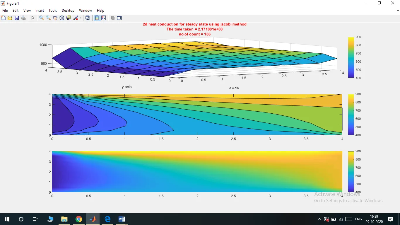
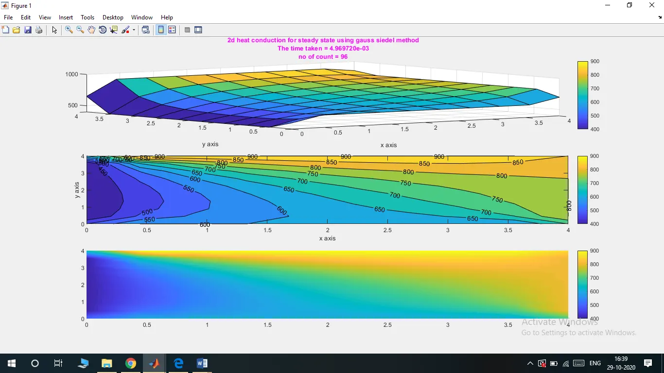
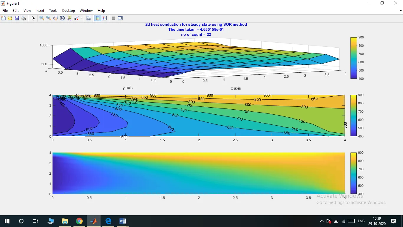
Matlab program for un-steady state explicit 2-dimensional heat conduction using iterative techniques:
close all
clear all
clc

h=4;
w=4;
n=10;
x=linspace(0,w,n);
y=linspace(0,h,n);

dx = x(2)-x(1);
dy=dx;
alpha=1.4;
t=40;
dt=0.03;
nt = t/dt ;
k3= (alpha*dt)/(dx)^2;
k4= (alpha*dt)/(dy)^2;

T= zeros(n);
T(1,2:n-1)=600;
T(n,2:n-1)=900;
T(2:n-1,1)=400;
T(2:n-1,n)=800;
T(1,1)=((600+400)/2);
T(1,n)=((600+800)/2);
T(n,1)=((900+400)/2);
T(n,n)=((900+800)/2);
Told = T;
toler=1e-4;
error=1;
omega=1.4;

iteration = input('The value of iteration')

tic
if(iteration==1)
     jacobi_iteration=1;
for k=1:nt
while error>toler
     for i=2:n-1
         for j=2:n-1
             term1=(Told(i-1,j)-(2*Told(i,j))+Told(i+1,j));
             term2=(Told(i,j-1)-(2*Told(i,j))+Told(i,j+1));
             T(i,j)= Told(i,j)+k3*term1+k4*term2
         end
     end
     error = (max(abs(Told(i,j)-T(i,j))));
     jacobi_iteration=jacobi_iteration+1;
     Told = T;
     end
end
time_unsteady1=toc
Output1 = sprintf('The time taken = %d',time_unsteady1)
 Output2 = sprintf('no of count = %d',jacobi_iteration)
 subplot(3,1,1)
 surf(x,y,T),colorbar,xlabel('x axis'),ylabel('y axis')
 colormap default
 title({'2d heat conduction for unsteady state using jacobi method';Output1;Output2},'color','m')
 subplot(3,1,2)
 contourf(x,y,T,'showtext','on'),colorbar
 subplot(3,1,3),pcolor(x,y,T),shading interp,colorbar
end

if(iteration==2)
    gs_iteration=1;
for k=1:nt
while error>toler
     for i=2:n-1
         for j=2:n-1
             term1=(T(i-1,j)-(2*Told(i,j))+Told(i+1,j));
             term2=(T(i,j-1)-(2*Told(i,j))+Told(i,j+1));
             T(i,j)= Told(i,j)+k3*term1+k4*term2
         end
     end
     error = (max(abs(Told(i,j)-T(i,j))));
     gs_iteration=gs_iteration+1;
     Told = T;
end
end
time_unsteady2=toc
 Output1 = sprintf('The time taken = %d',time_unsteady2)
 Output2 = sprintf('no of count = %d',gs_iteration)
 subplot(3,1,1)
 surf(x,y,T),colorbar,xlabel('x axis'),ylabel('y axis')
 colormap default
 title({'2d heat conduction for unsteady state using gauss siedel method';Output1;Output2},'color','m')
 subplot(3,1,2)
 contourf(x,y,T,'showtext','on'),colorbar
 subplot(3,1,3),pcolor(x,y,T),shading interp,colorbar
end

if(iteration==3)
    SOR_iter=1;
for k=1:nt
while error>toler
     for i=2:n-1
         for j=2:n-1
             term1=(T(i-1,j)-(2*Told(i,j))+Told(i+1,j));
             term2=(T(i,j-1)-(2*Told(i,j))+Told(i,j+1));
             T_gauss(i,j)= Told(i,j)+k3*term1+k4*term2
             T(i,j)=(((1-omega)*Told(i,j))+(omega*(T_gauss(i,j))))
             end
     end
     error = (max(abs(Told(i,j)-T(i,j))));
     SOR_iter=SOR_iter+1;
     Told = T;
end
 end
time_unsteady3=toc
 Output1 = sprintf('The time taken = %d',time_unsteady3)
 Output2 = sprintf('no of count = %d',SOR_iter)
 subplot(3,1,1)
 surf(x,y,T),colorbar,xlabel('x axis'),ylabel('y axis')
 colormap default
 title({'2d heat conduction for unsteady state using SOR method';Output1;Output2},'color','m')
 subplot(3,1,2)
 contourf(x,y,T,'showtext','on'),colorbar
 subplot(3,1,3),pcolor(x,y,T),shading interp,colorbar
end
PLOTS:
No of iteration taken by different iterative method for unsteady state heat conduction(Explicit):
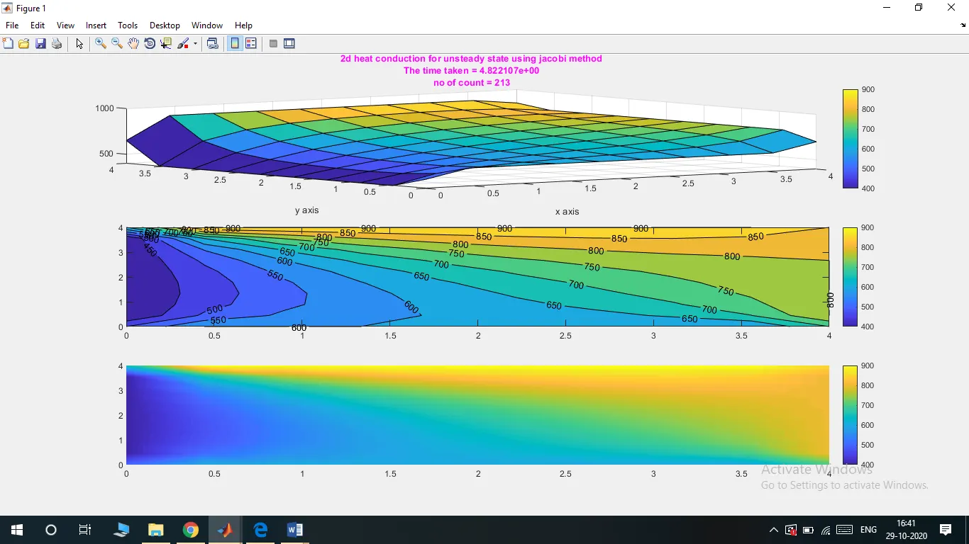
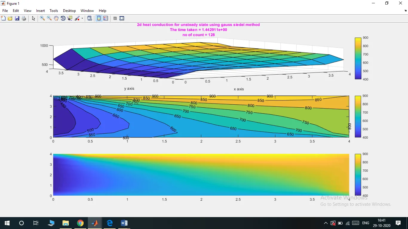
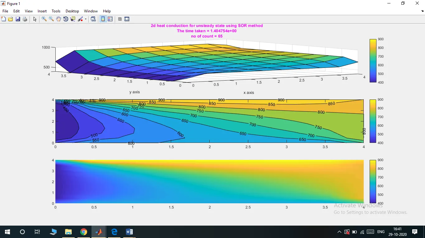
Matlab program for un-steady state implicit 2-dimensional heat conduction using iterative techniques:
close all
clear all
clc

h=4;
w=4;
n=10;
x=linspace(0,w,n);
y=linspace(0,h,n);

dx = x(2)-x(1);
dy=dx;
alpha=1.4;
t=40;
dt = 15;
nt = 1300;
k3= (alpha*dt)/(dx)^2;
k4= (alpha*dt)/(dy)^2;


T= zeros(n);
T(1,2:n-1)=600;
T(n,2:n-1)=900;
T(2:n-1,1)=400;
T(2:n-1,n)=800;
T(1,1)=((600+400)/2);
T(1,n)=((600+800)/2);
T(n,1)=((900+400)/2);
T(n,n)=((900+800)/2);
Told = T;
Tprev = Told;

omega=1.4;
toler=1e-4;
error=1;
iteration = input('The value of iteration')

tic
if(iteration==1)
     jacobi_iteration=1;
for L=1:nt
while error>toler
     for i=2:n-1
         for j=2:n-1
             term1=(1+2*(k3)+2*(k4))^(-1);
             term2= k3*term1;
             term3= k4*term1;
             H=(Told(i-1,j)+Told(i+1,j));
             V=(Told(i,j+1)+Told(i,j-1));
             T(i,j) = ((term1*Tprev(i,j))+(term2*H)+(term3*V))

         end
     end
     error = (max(abs(Told(i,j)-T(i,j))));
     jacobi_iteration=jacobi_iteration+1;
     Told = T;

end
T_prev = T;
end
time_unsteady_implicit=toc
 Output1 = sprintf('The time taken = %d',time_unsteady_implicit)
 Output2 = sprintf('no of count = %d',jacobi_iteration)
 subplot(3,1,1)
 surf(x,y,T),colorbar,xlabel('x axis'),ylabel('y axis')
 colormap default
 title({'2d heat conduction for implicit unsteady state using jacobi method';Output1;Output2},'color','r')
 subplot(3,1,2)
 contourf(x,y,T,'showtext','on'),colorbar
 subplot(3,1,3),pcolor(x,y,T),shading interp,colorbar
end

if(iteration==2)
    gs_iteration=1;
for L=1:nt
    while error>toler
     for i=2:n-1
         for j=2:n-1
             term1=(1+2*(k3)+2*(k4))^(-1);
             term2= k3*term1;
             term3= k4*term1;
             H=(T(i-1,j)+Told(i+1,j));
             V=(Told(i,j+1)+T(i,j-1));
             T(i,j) = ((term1*Tprev(i,j))+(term2*H)+(term3*V))

         end
     end
     error = (max(abs(Told(i,j)-T(i,j))));
     gs_iteration=gs_iteration+1;
     Told = T;

end
T_prev = T;
end
 time_unsteady_implicit1=toc
 Output1 = sprintf('The time taken = %d',time_unsteady_implicit1)
 Output2 = sprintf('no of count = %d',gs_iteration)
 subplot(3,1,1)
 surf(x,y,T),colorbar,xlabel('x axis'),ylabel('y axis')
 colormap default
 title({'2d heat conduction for implicit unsteady state using gauss siedel method';Output1;Output2},'color','b')
 subplot(3,1,2)
 contourf(x,y,T,'showtext','on'),colorbar
 subplot(3,1,3),pcolor(x,y,T),shading interp,colorbar
end


if(iteration==3)
    SOR_iter=1;
for k=1:nt

while error>toler
     for i=2:n-1
         for j=2:n-1
             term1=(1+2*(k3)+2*(k4))^(-1);
             term2= k3*term1;
             term3= k4*term1;
             H=(T(i-1,j)+Told(i+1,j));
             V=(Told(i,j+1)+T(i,j-1));
             T_gauss(i,j) = ((term1*Tprev(i,j))+(term2*H)+(term3*V))
             T(i,j)=(((1-omega)*Told(i,j))+(omega*(T_gauss(i,j))))
             end
     end
     error = (max(abs(Told(i,j)-T(i,j))));
     SOR_iter=SOR_iter+1;
     Told = T;

end
Tprev=T;
end
 time_unsteady_implicit2=toc
 Output1 = sprintf('The time taken = %d',time_unsteady_implicit2)
 Output2 = sprintf('no of count = %d',SOR_iter)
 subplot(3,1,1)
 surf(x,y,T),colorbar,xlabel('x axis'),ylabel('y axis')
 colormap default
 title({'2d heat conduction for implicit unsteady state using SOR method';Output1;Output2},'color','k')
 subplot(3,1,2)
 contourf(x,y,T,'showtext','on'),colorbar
 subplot(3,1,3),pcolor(x,y,T),shading interp,colorbar
end
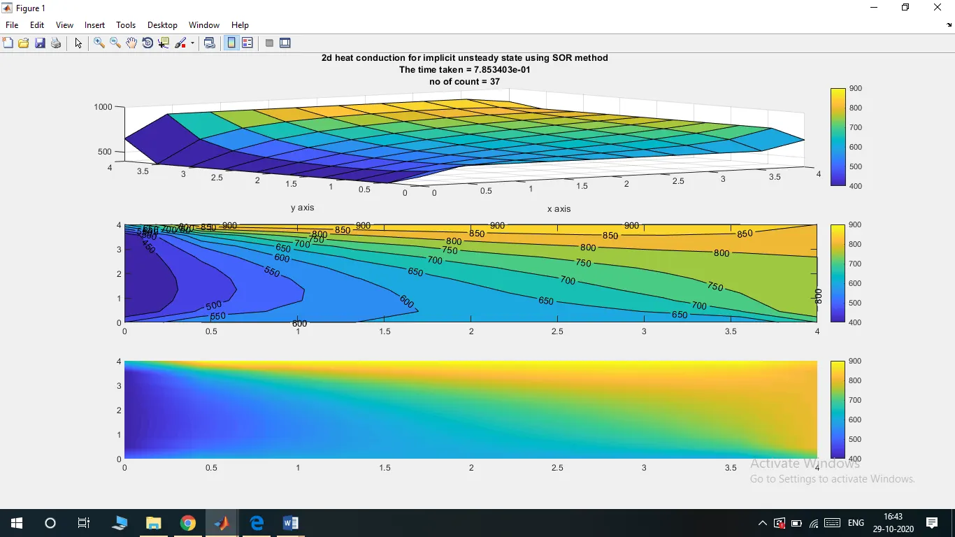
PLOTS:
No of iteration taken by different iterative method for unsteady state heat conduction(implicit):
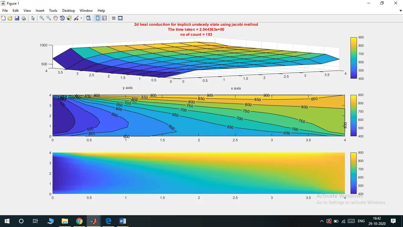
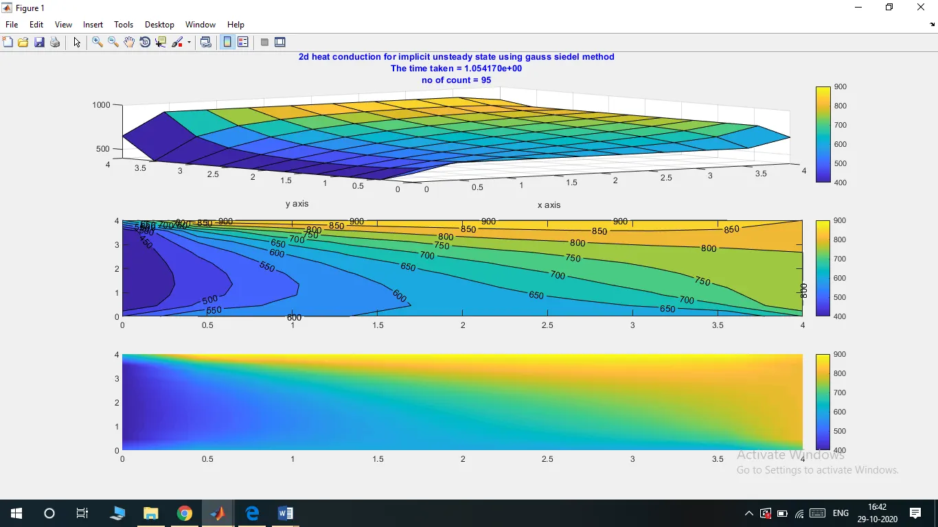
Tabulation of all the values for both explicit and implicit conditions:
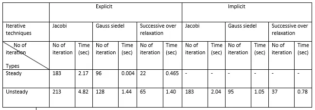
Convergence rate:
- In case of steady state 2-d heat conduction equation, the equation is simple also since its steady state equation its independent of time, and thermal diffusivity, and only dependent on spacial derivatives which makes it easy to solve, also no time marching is needed which in turn will get stable soon compared to unsteady state equation which comprises of time derivative, and also thermal diffusivity into account.
- When we compare unsteady explicit and implicit solution, the time taken by explicit solution may be greater or lesser it depends on the value of 'nt' no of time steps and 'dt', but in actual the explicit method take less time compared to implicit solution, because of less unknowns compared to implicit method ,but in case of implicit solution the simultaneous solution of unknown takes place at each grid point which results in greater number of equation whose solution will take greater time then Explicit method.
Differences in between implicit and explicit equation:
- Implicit is unconditionally stable, but explicit Simulations are only conditionally stable.
- Implicit scheme is Incremental as well as Iterative. But Explicit Scheme is only Incremental. Implicit scheme is a fighter, unless and until it is satisfied, it keeps on iterating. In case of explicit scheme. It keeps on Incrementing if or not the conditions of equilibrium are satisfied. This is why, the time used in Explicit should be very smaller. So, if in initial steps, an error happens, it keeps on magnifying.
- Implicit follows the Newton Raphson technique. But, Explicit follows the Euler Central Difference method. In the Newton Raphson method, there is a differentiation term
- In terms of Cost per Increment, it is costly for implicit and cheaper for Explicit. Because Implicit will cause Iterations until the conditions of equilibrium are fulfilled. This is why implicit increments are costlier than explicit increments.
- How does an unstable solution look like?
- At what CFL number does your solution become unstable ?
When we compare unsteady explicit and implicit solution, the time taken by explicit solution may be greater or lesser it depends on the value of 'nt' no of time steps and 'dt', but in actual the explicit method take less time compared to implicit solution, because of less unknowns compared to implicit method ,but in case of implicit solution the simultaneous solution of unknown takes place at each grid point which results in greater number of equation whose solution will take greater time then Explicit method.
In case if solution is unstable it does not converges and oscillates near actual points and never get ended.the unstability is due to use of wrong CFL number which should always be <1 =1 for explicit method .
In case if we use CFL number above '1' in case of explicit method we get unstable solution and it converges but the results we get are wrong.
The CFL number used in above explicit equation is greater then '1' hence getting no solution.
In case of implicit there is no such limit of using CFL number <=1 in some cases the CFL number can exceed to 30 we should just perform a trial and error and finalize a CFL method for this method.
The CFL condition is not an issue when both the convective and diffusive terms are evaluated at time t=t+1 (an implicit scheme).
Also if we use smaller CFL number in case of implicit solution many times it tends to unstable solution.
Conclusion:
From this challenge we were able to plot a results for 2-D heat conduction equation with different iterative techniques and able to find which iterative technique is better suitable to get equation converged in less number of iteration, and minimum time.
And from the results successive over relaxation is the iterative techniques which is more suitable.