Week 9: Project 1 - Surface preparation and Boundary Flagging (PFI)
Simulating Spart Ignited Port Fuel Injection Engine (Part-1) Geometry preparation
Aim:- Geometry (Surface) preparation and Boundary Flagging of Spart Ignited Port Fuel Injection Engine.
Objectives:
- Splitting it into meaningful boundaries.
- Flagging the boundaries.
- Creating Regions.
Port fuel-injection:-
Port fuel injection systems long ago replaced carburetors in cars because of their efficiency and lower maintenance requirements. But now, automakers are moving towards even more efficient direct injection. With port fuel injection, gasoline is sprayed into the intake manifold, where it mixes with air, and then is sucked down into the cylinders. Direct injection places an injector on each cylinder, spraying gasoline into the cylinder itself. Direct injection leads to more efficient engines, as the gasoline-air mixture burns more completely. The individual injectors also ensure that each cylinder gets the same amount of fuel, and the spray can be more precisely timed.
Flow simulation in CONVERGE done in 3 steps:
- Geometry preparation and Case setup :
- We use Converge GUI(Graphical User Interface) to set up the case and export input files.
- Solving the problem using input files:
- These input files are solved by Converge in the Terminal (Command-line interface). We USed Cygwin for the command line terminal.
- Post-processing results:
- We convert our solution into Paraview binary format to post-process the results in Paraview
Geometry(Surface) preparation in CONVERGE CFD:
- Geometry preparation:
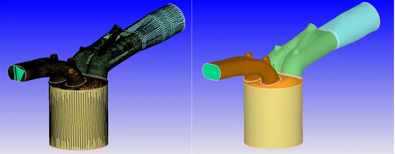
- Import the ".STL" "Standard Triangle Language" file of the Spark Ignited Engine.
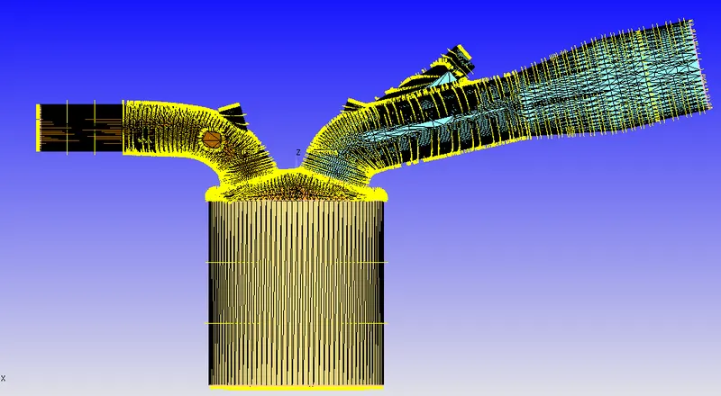
- Drag and drop the "IC_engine.STL" file. Geometry has imported into the converge.
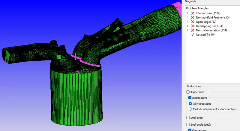
- Run The Diagnosis text to find any problem triangles.
- This geometry has multiple errors. at this stage, it is a bit difficult to eliminate these errors.
- In order to eliminate these errors easily, we have to flag the boundaries and regions. Later, we can hide these boundaries and regions to fix the problem triangles.
- Boundary Flaging:
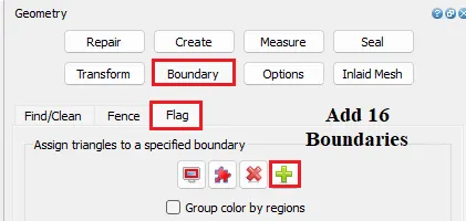
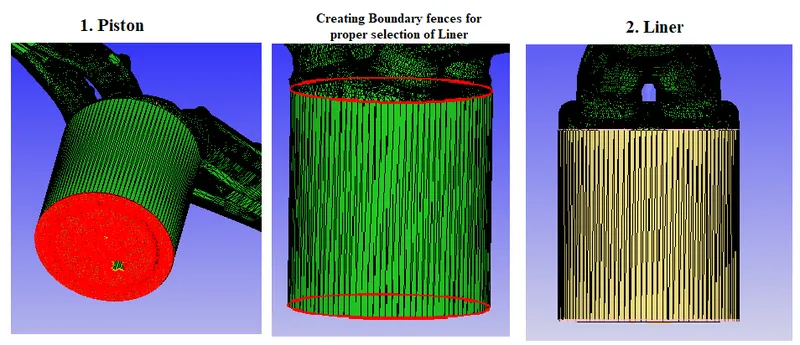
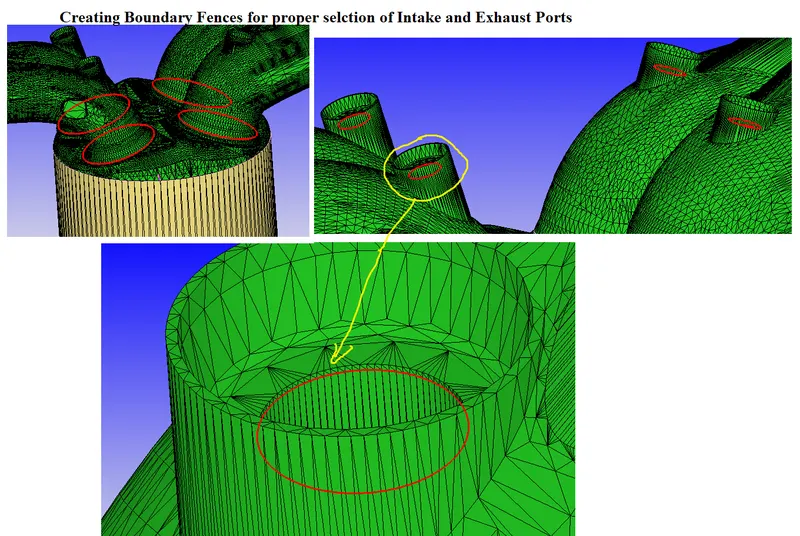
- Create boundary fences were ever required for proper section of triangles.
- By default In CONVERGE, all the surfaces are made up of triangles we have to select respective triangle faces for the boundary.
- Piston & liner:-
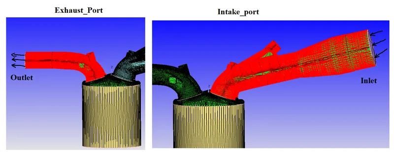
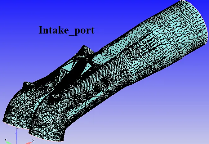
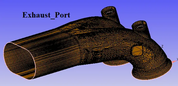
- Intake & Exhaust Ports:-
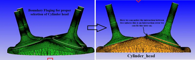
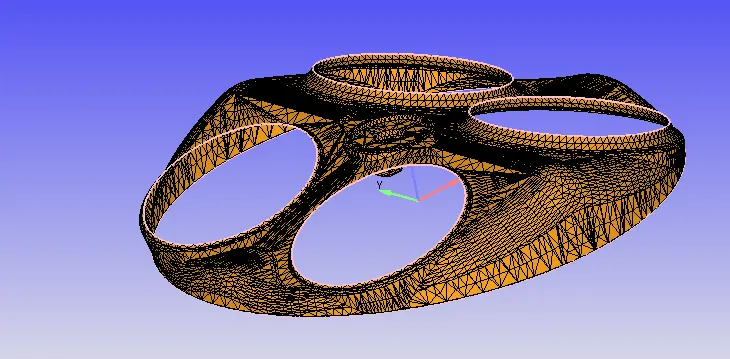
- Cylinder head:-
- Hide all the Boundaries so that it will allow us to select internal components easily.
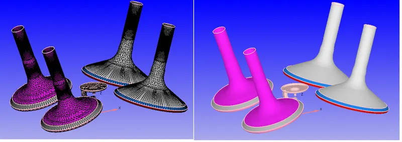
- Intake & Exhaust Valves:-
- Hiding all other Named Boundaries and splitting valves into three components because :
- We use events to control flow between regions by splitting the valves we can create events easily.
- By splitting the valve we can add an additional embedding mesh layer over it. So, that it can resolve the flow field perfectly.
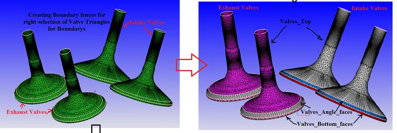
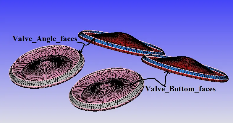
- Hiding all other Named Boundaries and splitting valves into three components because :
- Spark plug and terminal:-
- Isolate the Cylinder head.
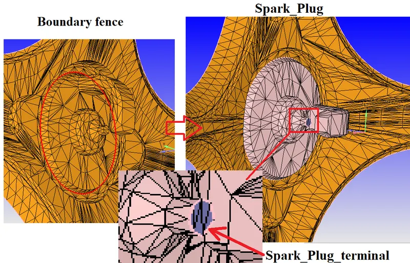
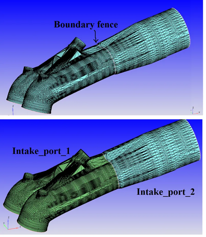
- Splitting Intake port:-
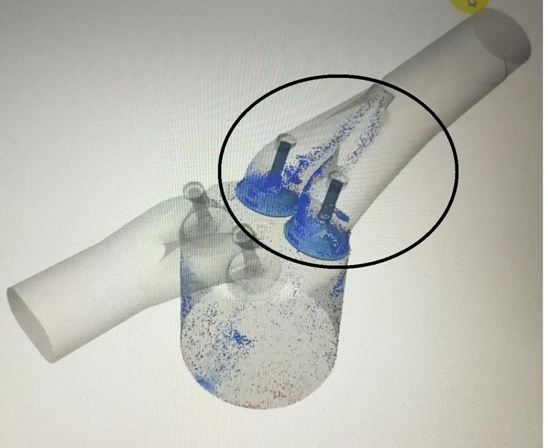
- Splitting Intake port into two pieces for providing better initial conditions
- When the intake port is in the closed position spray particles still exist in the first half part of the intake port which is closer to the cylinder.
- So we have to initialize some amount of fuel in the intake port closer to the combustion chamber.
- When the intake port is in the closed position spray particles still exist in the first half part of the intake port which is closer to the cylinder.
- Splitting Intake port into two pieces for providing better initial conditions
- Fixing triangular problems:
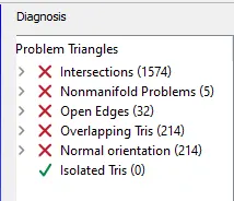
- Now we are more accessible to resolve the issues we can hide any boundary that we want to hide.
- Intersections:
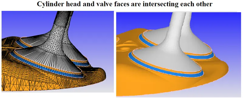
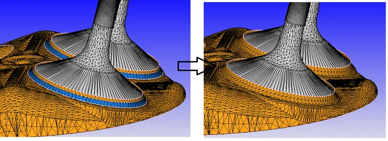
- To resolve this issue we have to move the valve downwards along the normal direction so that there is no more intersection between faces.
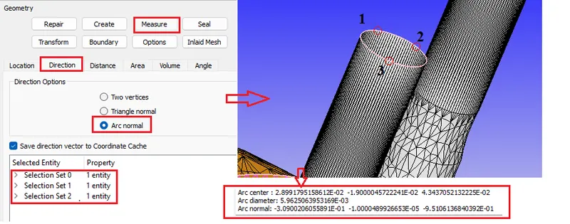
- finding normal direction of valve.
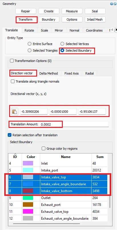
- Use the translate option to move the valve downwards.
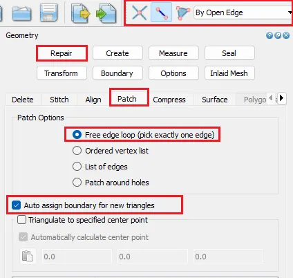
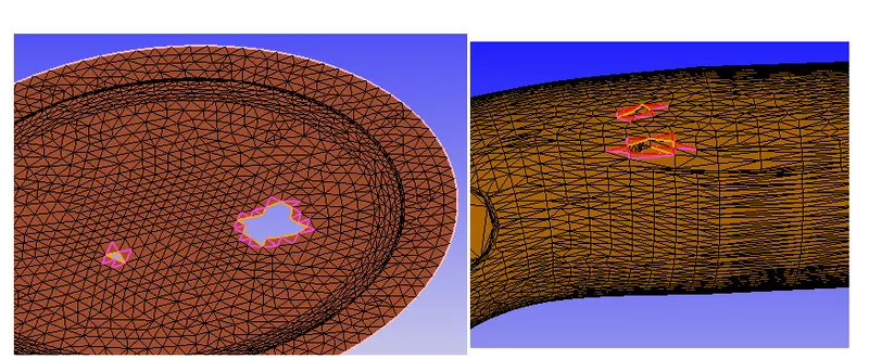
- Open Edges:-
- use Patch option in Repair to close the open edges.
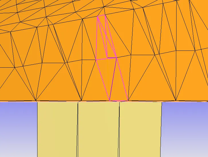
- Overlapping tris:-
- Delete the overlapping triangles & add where ever required.
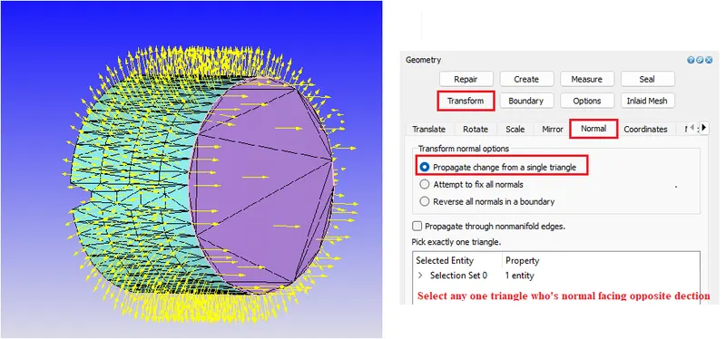
- Normal orientation:-
- All the face normal direction should be facing towards the fluid domain.
- If any normal facing outwards, we have to transform the normal's direction into the fluid domain.
- Final Setup:
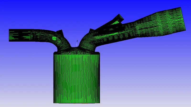
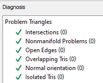
- Run Final Diagnosis: No issues found
---------------------------------------------------------------------------------------------------------------------------------------------
Case Setup:
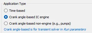
- Application type:
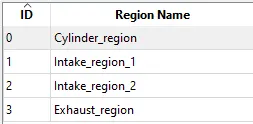
- Creating Regions:
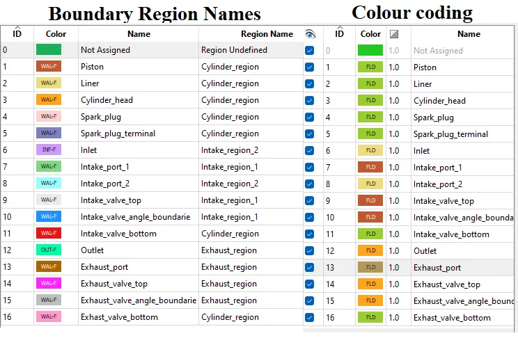
- Creating 4 regions
- Assigning these regions to the respective boundaries
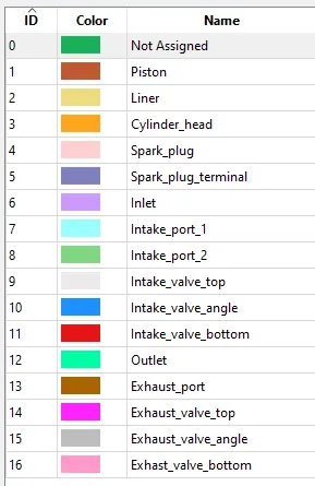
- from the below picture, we can see the color codes of boundaries and regions.
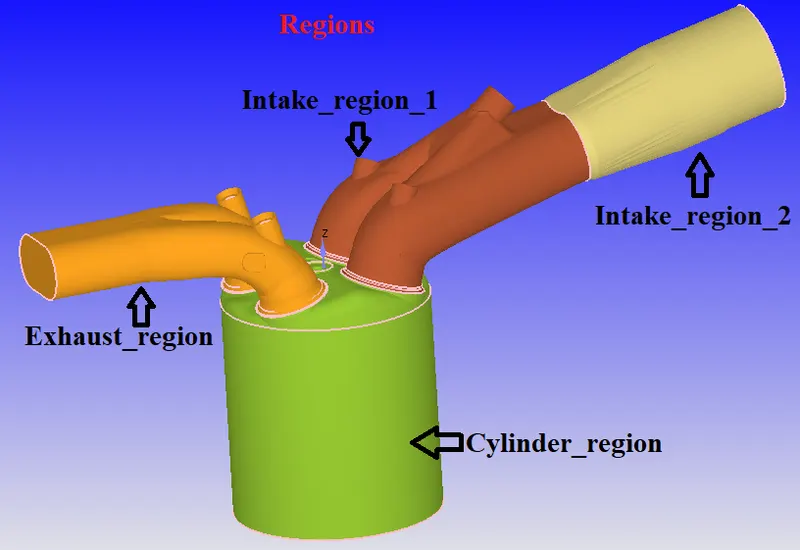
- Creating 4 regions
- Materials:
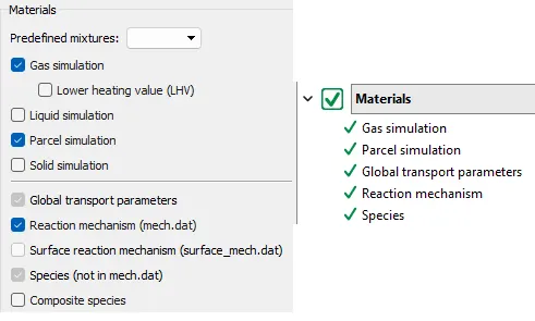
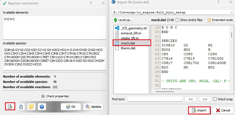
- "mech.dat" file contains gas-phase chemical reactions.
- "therm.dat" file contains the thermodynamic properties of each gas phase.
-
- Gas Simulation
- Importing Gas Thermodynamic data
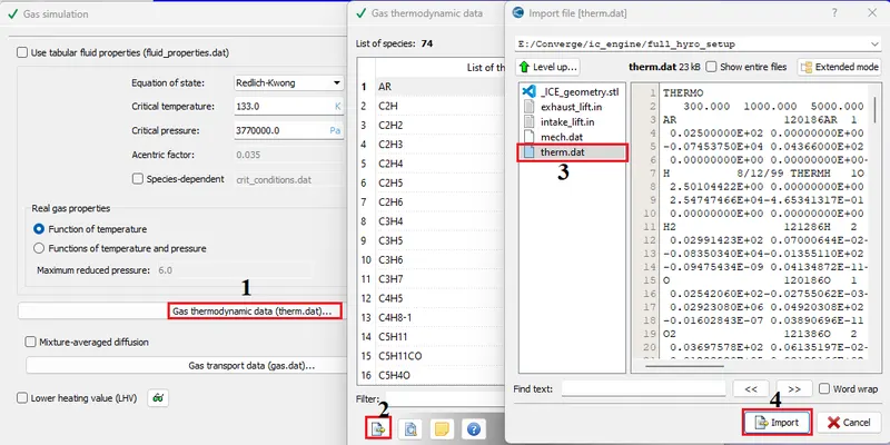
- Global transport properties ==>> Default
- Reaction Mechanism:-
- We need to select a reaction mechanism that is compatible with gasoline. JIA PRF(Primary reference fuel) best compactable mechanism for gasoline engines.
- Reaction mechanism => import "mech.dat" file.
- Parcel Simulation :
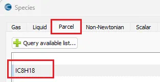
- We have to select the right species for our parcel is made up of. if we don't find the exact fuel species that we are looking for we can use the species whose physical properties match with our actual fuel physical properties.
- IC8H18_isooctane has physical properties which are very much closer to gasoline fuel.
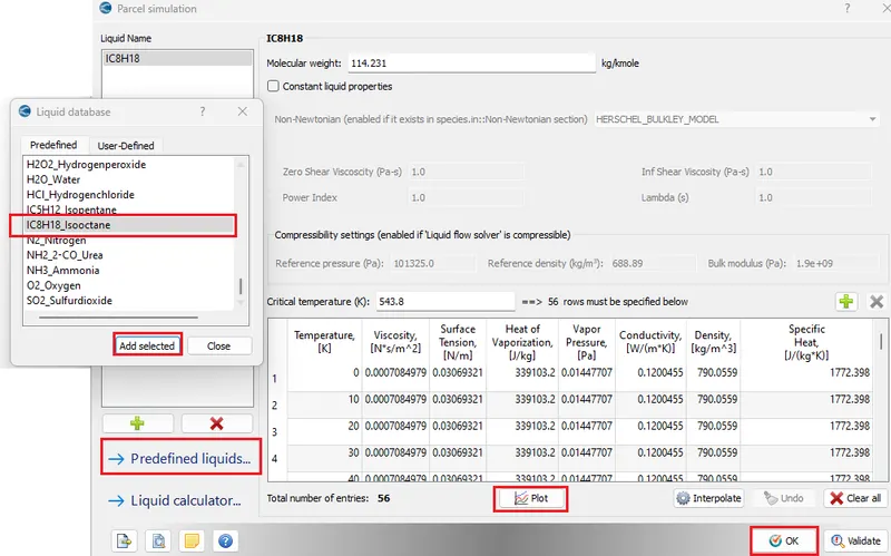
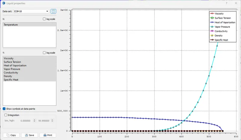
- Species:
- We have to add IC8H18 in the parcel section.
- We have to add IC8H18 in the parcel section.
- Gas Simulation
- Simulation Parameters:
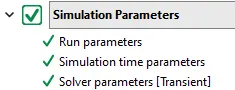
- Run Parameters:
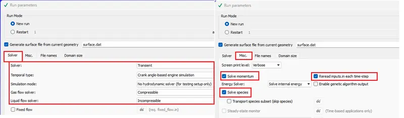
- Transient, Crank angle based engine simulation with No Hydrodynamic solver.
- In the No Hydrodynamic case, no equation is going to solve. for this case we are interested in the Mesh generation part, Before every large simulation which contains moving parts, we have to run a no-hydro case to check any errors like intersections, open edges etc. By no-hydro simulation, we can visualize the detailed movement of every moving part.
- Gas is compressible and liquid is incompressible.
- Solve momentum, & Species.
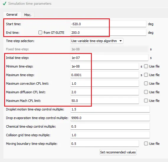
- Simulation Time Parameters:
- Total run time = one cycle = 720 degrees
- Start at suction stroke -520 degrees till exhaust stroke completes -520+720 = 200degrees
 \
\
- Solver Parameters:
- Run Parameters:
- Initial Conditions and events:
- Stochiometric composition:
- `C_8H_18 + 12.5(O_2+3.76N_2) => 8CO_2 + 9H_2O+41N_2`
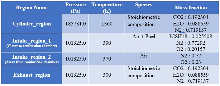
- Regions and initialization:
- Before starting the simulation we have to initialize the regions in the simulation.
- Events:
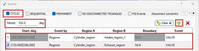
- During the Engine operation, the Intake port & Cylinder, are connected during suction and disconnected for the rest of the period. Similarly, the Exhaust port & Cylinder are connected during Emission and disconnected for the rest of the period.
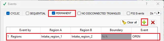
- For better initialization and meshing, we split out Intake port into 2 regions we have to always connect these regions.
- Above mentioned two conditions can be achieved by creating events by this we can connect and disconnect the regions.
- Cyclic event:
- The first situation can be handled by creating Cyclic events by this cyclic event we can connect and disconnect regions over the span of a period.
-
- Permanent event:
- The second situation can be handled by creating Permanent events by this permanent event we can connect or disconnect regions throughout the simulation.
- Cyclic event:
- Above mentioned two conditions can be achieved by creating events by this we can connect and disconnect the regions.
- Regions and initialization:
- Initializing regions:
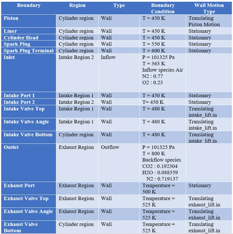
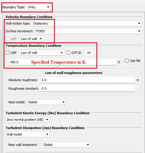
- All Stationary Walls :
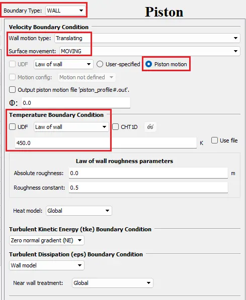
- Piston:
- The Piston is under Translating motion, we have pre-defined piston motion that can be enabled for piston motion for this Piston wall boundary.
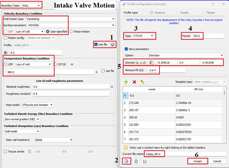
- Intake Valve:
- The intake valve is split into 3 sections top, angle, and bottom all three are translating walls. The movement of all these valves is User-specified.
- use the "intake_lift.in" file to assign valve motion during cyclic motion, period: 720 degrees crank angle.
- The direction of motion is the same as the axis of the valve. Measure => Direction => Arc Normal.
- The minimum lift was set to 2e-4. It is the minimum gap between Valve and the cylinder head. if we completely close the gap, the mesh gets overlapped causing problems during simulation i.e, we have to maintain the minimum gap between faces.
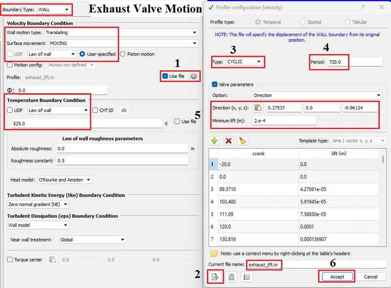
- Exhaust Valve:
- The intake valve is split into 3 sections top, angle, and bottom all three are translating walls. The movement of all these valves is User-specified.
- use the "exhaust_lift.in" file to assign valve motion during cyclic motion, period: 720 degrees crank angle.
- The direction of motion is the same as the axis of the valve. Measure => Direction => Arc Normal.
- The minimum lift was set to 2e-4. It is the minimum gap between Valve and the cylinder head. if we completely close the gap, the mesh gets overlapped causing problems during simulation i.e, we have to maintain the minimum gap between faces.
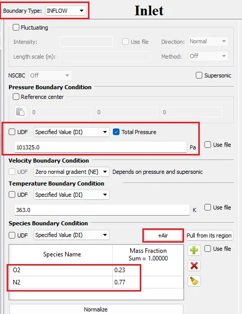
- Inlet:
- Through the inlet, air flows into the cylinder at atmospheric pressure at 363K. Add air mas fractions in Species boundary condition.
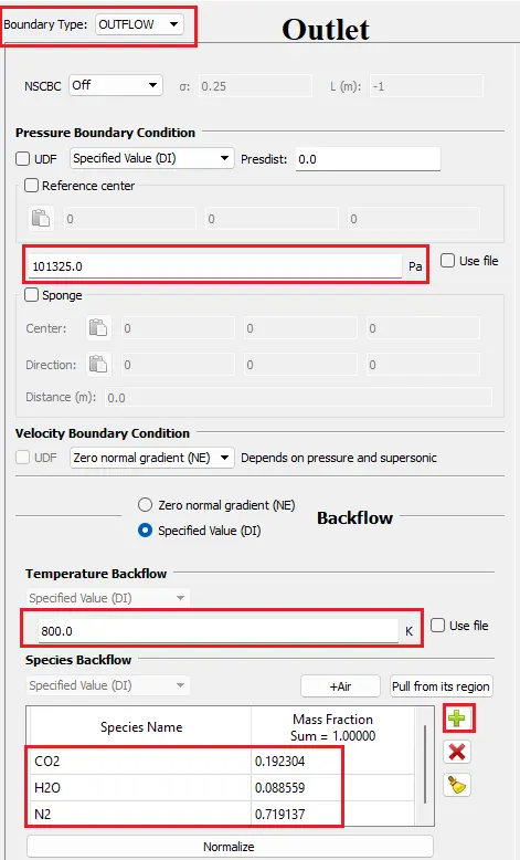
- Outlet:
- Through Outlet, combustion products flow out of the cylinder to atmospheric pressure at 800K. Add mas fractions of products of combustion in Species boundary condition.
- All Stationary Walls :
- Physical Models:
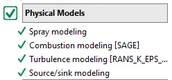
- In Physical models, we have to enable Spray modeling, Combustion modeling, Turbulence modeling & Source/Sink modeling.
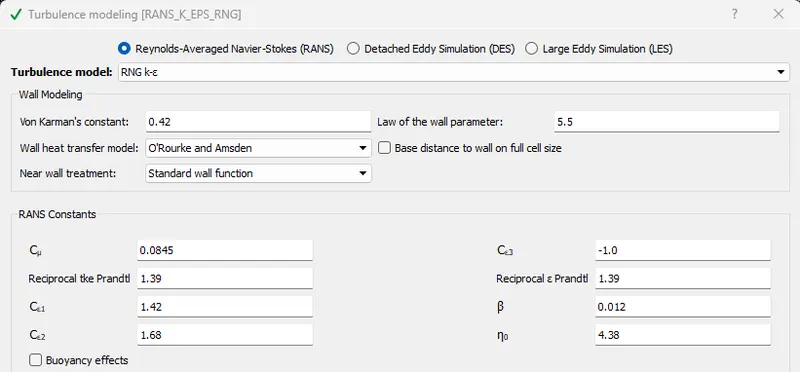
- Turbulence modeling :
- RNG K-`epsilon`
- Spray Modeling:
- General:
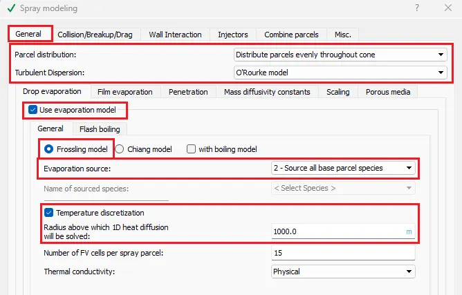
- IC8H18 parcels are evenly distributed evenly through the cone
- We have turbulence in the gas phase this turbulence fluctuations can affect the droplet characteristics. Typically for gasoline engines, the O'Rourke model is preferred.
- Our IC8H18 fuel is evaporated into IC8H18 vapor.
- Basically, our fuel parcels are in a spherical shape, the outside of the sphere is much hotter than the inside of the sphere. We can basically discretize the droplet into a number of spherical finite volume cells and solve heat ODE equations in all of those individual finite volume cells. In our case, we are not interested in solving this because we don't need that level of accuracy that's why we are considering our droplets are of one temperature. It can be achieved by using a larger value for the radius so that ode is never solved. ODE is solved when the parcel radius is more than the specified radius.
- Collision/Breakup & Wall Interaction:
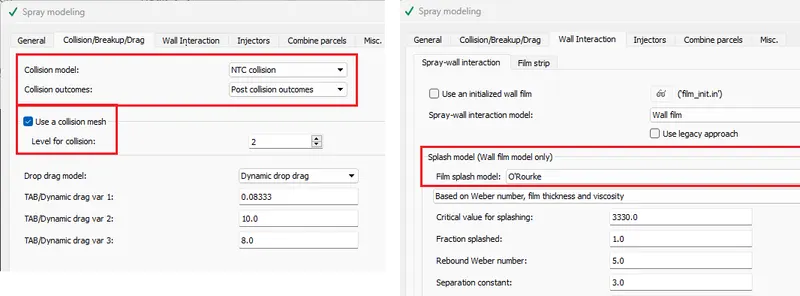
- NTC Collision model, Post Collision outcomes.
- Use collision mesh to avoid grid effects.
- Injectors:
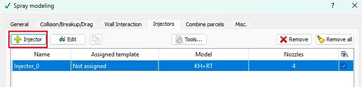
- Adding injector.
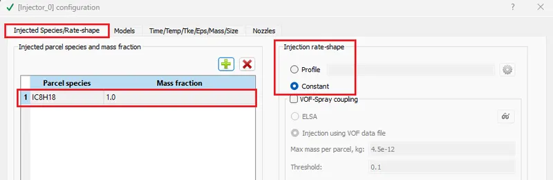
- Injector Species Rate shape = constant.
- Injector Species = IC8H18, Rate shape = constant.
- Models:
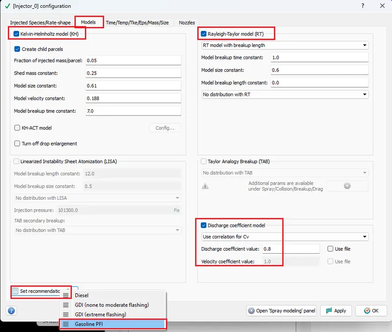
- Kelvin-Helmholtz & Rayleigh-Taylor are the Popular models used for solid cone sprays.
- Set recommended values for gasoline fuel.
- These Constant values control how your parcel going to break up.
- Temp/time/mass/size
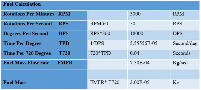
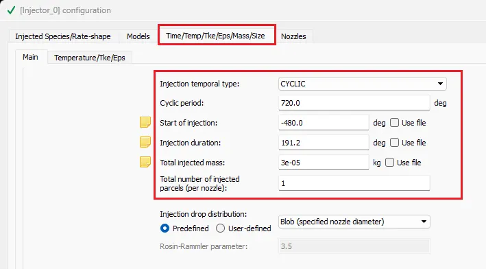
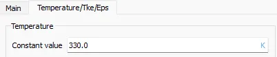
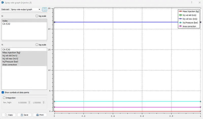
- In the case of the engine, fuel spray does not take place at every second it takes place at every cycle. This flow rate can be converted into absolute mass
- Nozzles:
- We have 4 nozzles attached to the one injector.
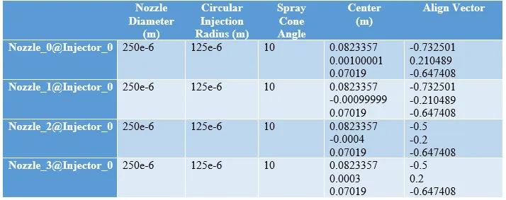
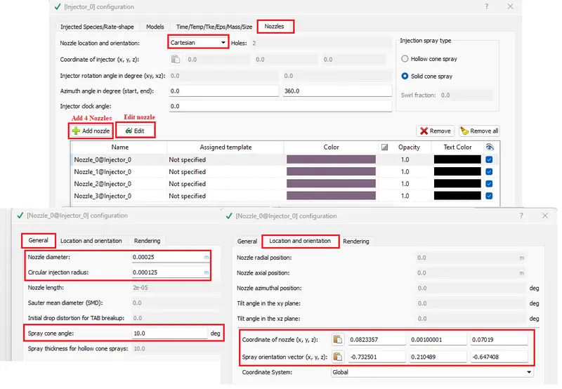
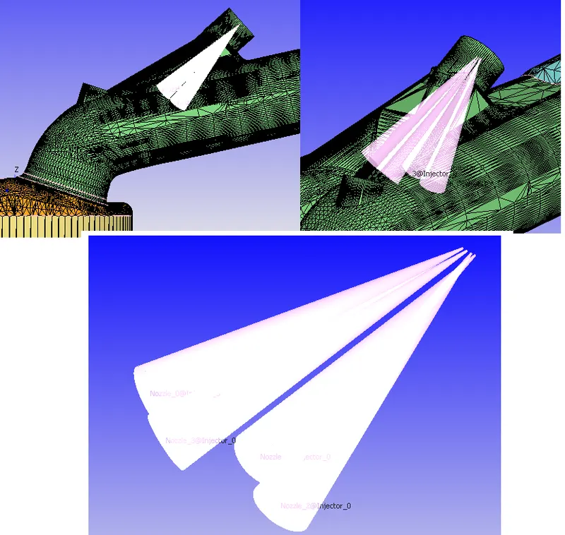
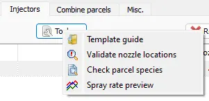
- Validate Nozzle location all nozzles should be inside computational domain.
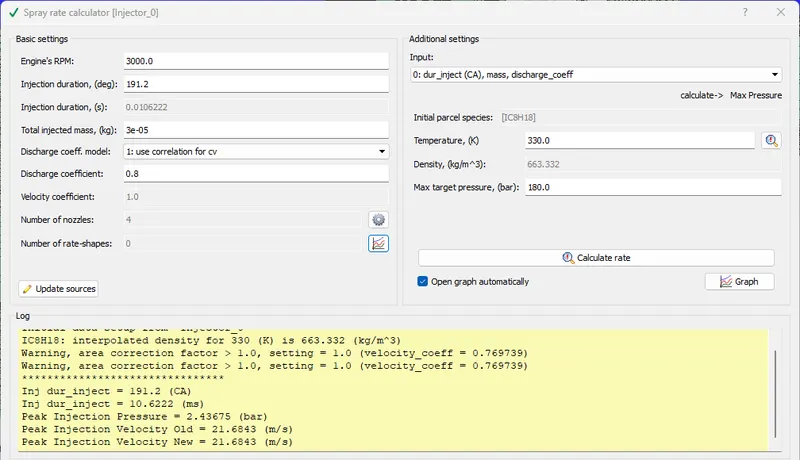
- Adding injector.
- General:
- Combustion modeling:
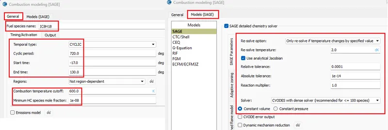
- SAGE combustion Model is used to speed up the combustion calculations.
- Combustion starts a few crank angles before the spark. Spark starts at -15 deg combustion start at -17.
- Combustion ends when the exhaust valve opens 130 deg.
- Source/Sink modeling:
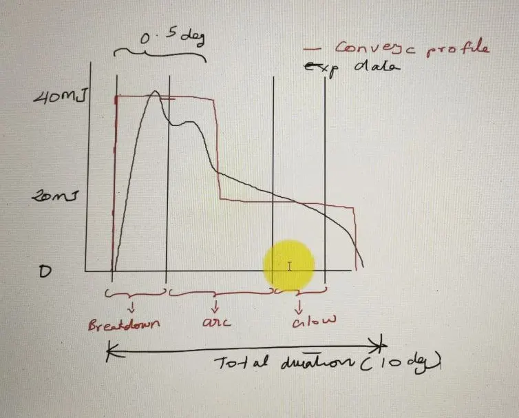
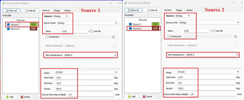
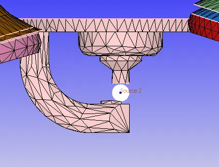
- The spark plug can be introduced by adding energy sources this will increase the temperature of the species in the species transport equation this temperature going to be introduced as source terms and responsible for combustion.
- The source is spherical in nature.
- During the Breakdown phase, we need more energy to conduct between spark gap. After the breakdown, we need litter more energy to keep the conduction going on. This can be achieved by adding two energy sources first energy source produces 0.02J of energy for 0.5deg and the second source produces another 0.02J for the entire length. So, during the breakdown phase, source 1 & 2 combinedly produces 0.04J after that source 2 maintains 0.02J energy.
- Turbulence modeling :
- Grid Control:
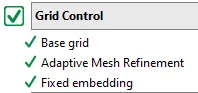
- The meshing part can be done through Grid control.
- Base grid:
- Setting base grid size to 0.004 m or 4 mm

- Fixed Embedding:
- We don't need highly refined mesh in the entire domain this will leads to more computation time to solve and every cell, on the same way we cannot use coarse mesh which will take us to inaccurate and wrong results. To overcome this problem we are going to refine the mesh in particular zones or areas.
- Permanent Boundary based Embedding over valve angle faces:
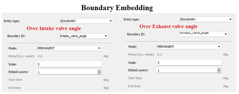
- The main reason for doing this embedding is because we are using a base mesh size equal to 0.004 meters and the minimum lift was set to 0.002 meters. It is hard to get more cells in the gap, based on the 30% of criteria created cells get paired to each other by this we lose our accuracy. To overcome this we are using boundary-based permanent embedding over Inlet and Exhaust valve angle faces with a scale of 3.
- `text(Cell size) = text(Base mesh size)/2^(text(Scale)) = 0.004/2^(3)=0.0005 text( meters)`
- Permanent Region-Based Cylinder Embedding:
- Finer mesh inside the Cylinder:
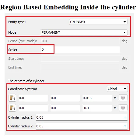
- The combustion takes place inside the cylinder so we need more refined mesh inside the cylinder. For this, we are going to use region-based embedding inside the cylinder with an element size of 0.001 meters. The scale of 2 gives 1 mm cells for a base mesh size of 4mm.
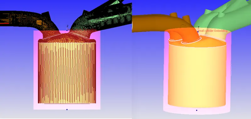
- Corser mesh refinement near to the Cylinder:
- Near to the Cylinder we don't need a high level of refinement so we can go with 2 mm cells near to the cylinder. The scale of 1 gives 2 mm cells.
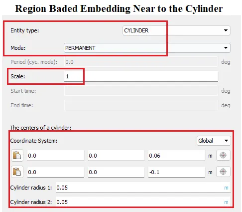
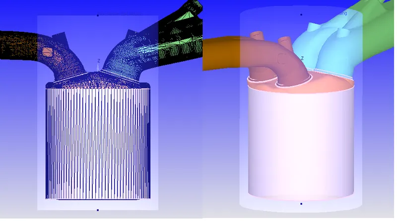
- In Region-Based embedding, our main aim is to cover the geometry that we want to mesh. If there are a lot of unnecessary volumes we are embedding it is absolutely fine as there is no geometry there no cells will be created.
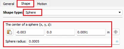
- Region-Based Sphere Embedding around source terms:
- We added energy in the form of source terms we have to make sure that we have less numerical diffusion can be achieved by adding more refinement near around sources.
- When the spark is suddenly introduced just at the instant there is no proper refined mesh to calculate gradients accurately. after that Temprtature AMR refines mesh based on temperature curvature.
- we are introducing a highly refined mesh that can be last for a few crank angles will calculate gradients accurately
- Refinement starts before spark ignition and lasts until the end of ignition.
- Sphere radius of 0.001m around the source is refined up to the scale of 5. cell size = 4/32=1/8 =0.125 mm
- Sphere radius of 0.003m around the source is refined up to the scale of 3. cell size = 4/8=1/2 =0.5 mm
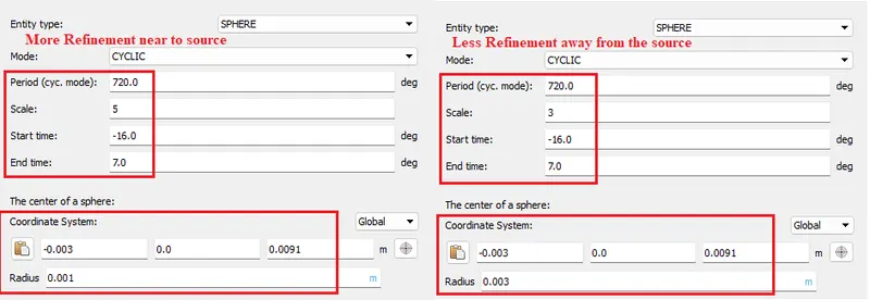
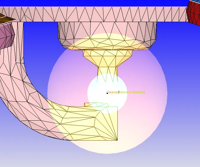
- Region-Based Injector Embedding around fuel injector spray:
- In the injector cone area, our spray parcels are atomized some of them are vaporized to capture right physics we need refinement.
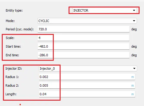
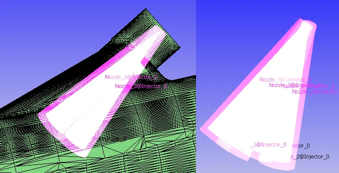
- Finer mesh inside the Cylinder:
- Permanent Boundary based Embedding over valve angle faces:
- Adaptive Mesh refinement (AMR):
- In Adaptive Mesh refinement mesh gets auto-refined according to the condition given.
- here we are specifying the maximum number of cells that can be reached after refinement is 200,000 cells.
- firstly we have to shift the Volumetric_region in available regions to active regions.
- For this case, we are using Velocity & Temperature based AMR so that we can monitor the curvature of Velocity and temperature
- Embed type: Sub-grid Scale (SGS)
- we have to enter magnitude for sub-grid criterion. for example, if we enter Sub-grid criterion = 0.001 mesh gets auto refined in the region where the variable difference between `N_(th)` cell and `(N-1)_(th)` cell is greater than SGS criteria.
- Max embedding level is used to calculate the size of the refined cell.
- `text(Grid size)=text(Base grid size)/2^text(Embed level)`
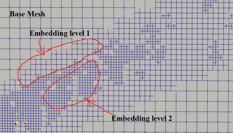
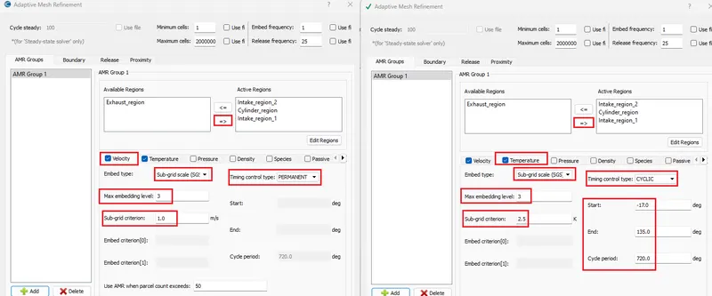
- Velocity AMR is permanent and continuous throughout the simulation.
- Temperature AMR is cyclic in nature starting just before the spark starts and ending when combustion ends.
- We don't need highly refined mesh in the entire domain this will leads to more computation time to solve and every cell, on the same way we cannot use coarse mesh which will take us to inaccurate and wrong results. To overcome this problem we are going to refine the mesh in particular zones or areas.
- The meshing part can be done through Grid control.
- Output/Post-Processing
- Post Variable selection: select the variables to be monitored for post-processing.
-
S.No Typical variables Geometry/Location 1 Density Region ID 2 Pressure 3 Temperature 4 Velocity 5 Mesh Quality 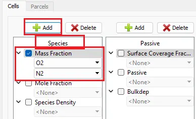
-
S.No Turbulence 1 Dissipation Rate of tke (eps) 2 Turbulent Kinetic Energy(tke) 3 Turbulent Viscosity 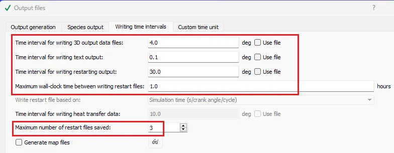
-
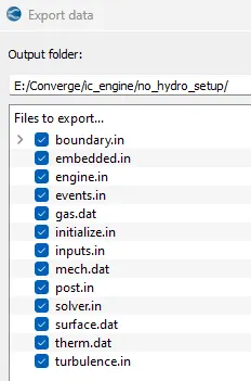
- Exporting Input files:
- Export the input files
- Export the input files
- Post Variable selection: select the variables to be monitored for post-processing.
-
Solving Channel Flow in Cygwin:
- Go to the directory where input files are exported
- Make mpiexec.exe & converge.exe files globally available.
- "mpiexec.exe -n 4 converge.exe restricted logfile &"
- Use above mentioned line to start calculation in the background
- mpiexec.exe & converge.exe are executable applications to solve the problem
- -n 4:- number of processors
- restricted:- my license is a restricted one.
- logfile:- creates temporary memory to save data with name as logfile at a particular iteration
- & :- To run Calculation in Background
- "tail -10 logfile" command is used to view the last 10 lines of the log file.
- "mpiexec.exe -n 1 post_convert_30_serial_64" command used to convert output files to paraview binary format, so that they can be processed in the paraview.


Post Processing and Results from Paraview:-
- open "..vtm" group file in paraview. This group contains all the solution files.
- use the slice tool to create a plane on which we can visualize the mesh at different crank angles.
- Slicing the geometry
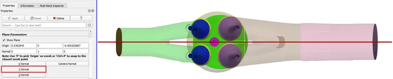
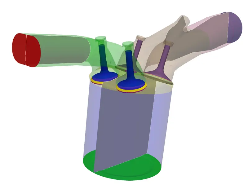
- Slice 1:
- Normal to Y-axis and splitting geometry into two equal half's.
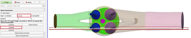
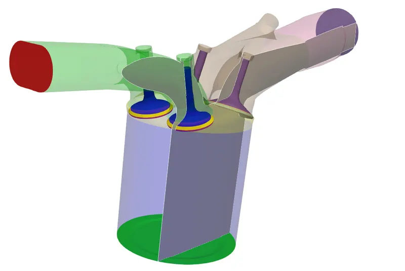
- Slice 2:
- Normal to Y-axis with offset y distance = -0. 19 which will split the valves .
Mesh structure at different crank angles:
- Crank angle = 0
- Crank angle = 45
-
- Crank angle = 90
- Crank angle = 135
- Crank angle = 180
- Crank angle = 225
- Crank angle = 270
- Crank angle = 315
- Crank angle = 360
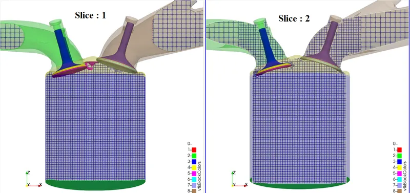
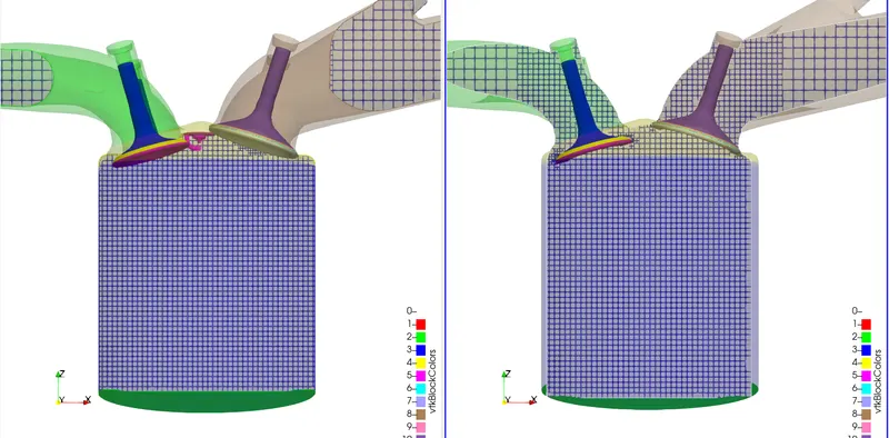
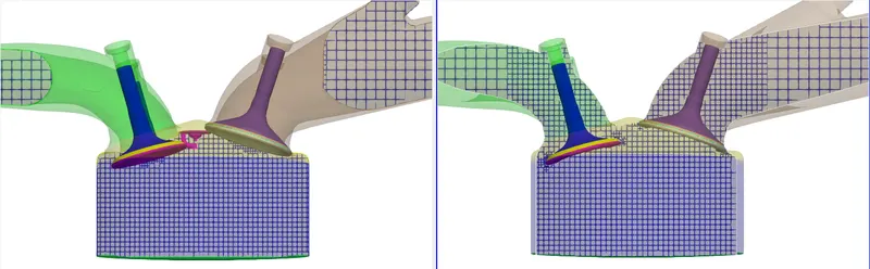
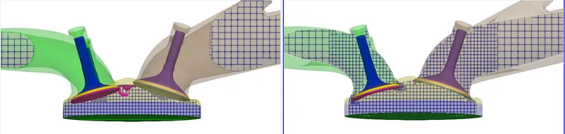
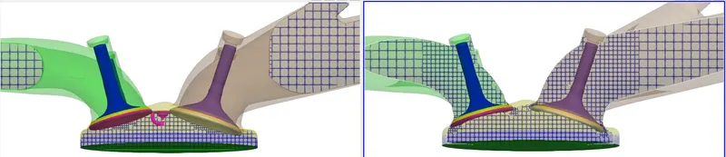
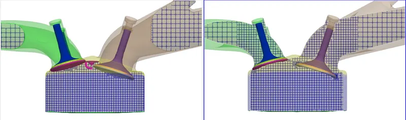
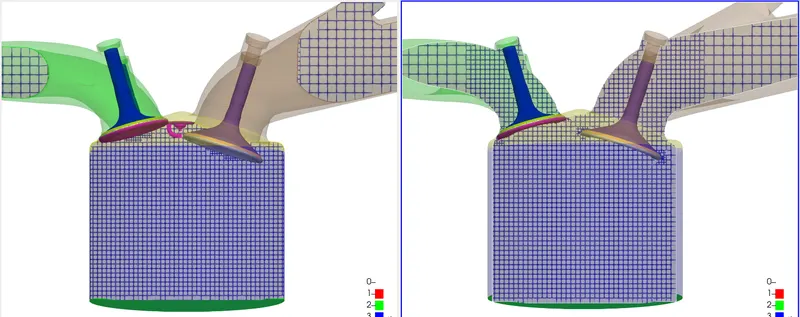
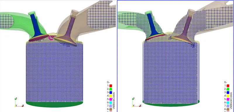
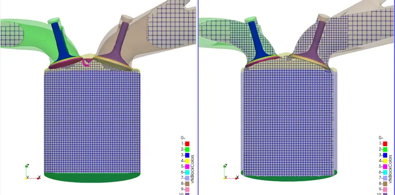
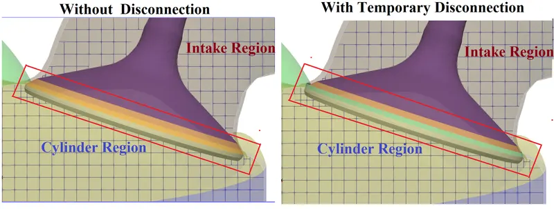
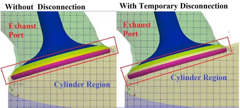
During the engine operation valves have to open and close to supply the air-fuel mixture and to remove exhaust gases. This moment can be achieved by adding lift profiles to the valves. When the valves are under closed conditions valve angle faces must be attached to the cylinder head to make a perfect seal between the cylinder region and the Intake/Exhaust region. From the simulation point of view if this really happens this leads to getting overlapping and intersection triangles causing triangle problems(error). To tackle this issue we are going to move the valve bit down by 0.02 mm this avoids the formation of a triangle problem but introduces a new problem called leakage into the cylinder region. To avoid leakage from 0.02mm gap should be closed when the valve is in the closed position and has to open when the valve is in the open position. This temporary closing and opening can be achieved by creating something called valve events. These valve events temporarily disconnect the cylinder region and intake/Exhaust ports when the valve is in closed condition and connect when the valve is in open condition. In the no-hydro simulation, we have to check whether these are connecting and disconnecting properly.