Analyze Trace Heating of a Printed Circuit Board (PCB) in Electronics

AIM: Analyze Trace Heating of a Printed Circuit Board (PCB) in Electronics.

Introduction:

Printed circuit boards (PCBs) are the boards that are used as the base in most electronics – both as a physical support piece and as the wiring area for the surface-mounted and socketed components.

There are several different types of circuit boards, each with its own particular manufacturing specifications, material types, and usages:

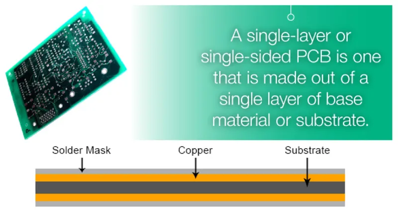
i) Single-layer PCB - A single-layer or single-sided PCB is one that is made out of a single layer of base material or substrate. One side of the base material is coated with a thin layer of metal.

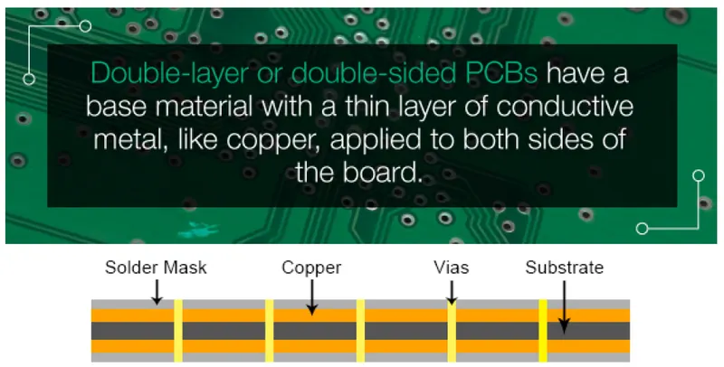
ii) Double-layer PCB - Double-layer or double-sided PCBs have a base material with a thin layer of conductive metal, like copper, applied to both sides of the board. Holes drilled through the board allow circuits on one side of the board to connect to circuits on the other.

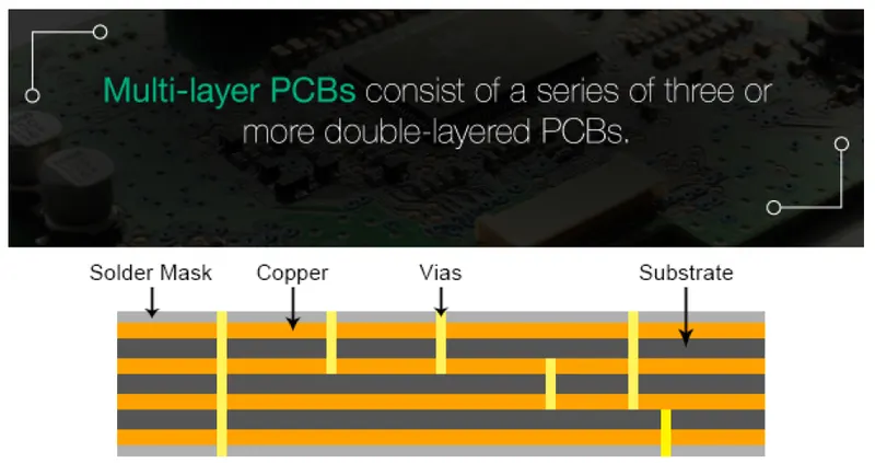
iii) Multi-layer PCB - Multi-layer PCBs consist of a series of three or more double-layered PCBs. These boards are then secured together with a specialized glue and sandwiched between pieces of insulation to ensure that excess heat doesn't melt any of the components.

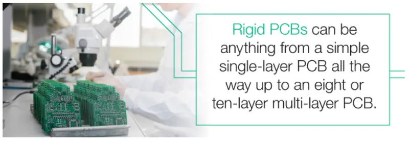
iv) Rigid PCB - Rigid PCBs are made out of a solid substrate material that prevents the board from twisting. Possibly the most common example of a rigid PCB is a computer motherboard. The motherboard is a multilayer PCB designed to allocate electricity from the power supply while simultaneously allowing communication between all of the many parts of the computer, such as CPU, GPU and RAM.

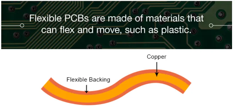
v) Flexible PCB - Flexible printed circuit boards is made of materials that can flex and move, such as plastic. Like rigid PCBs, flexible PCBs come in single, double or multilayer formats.

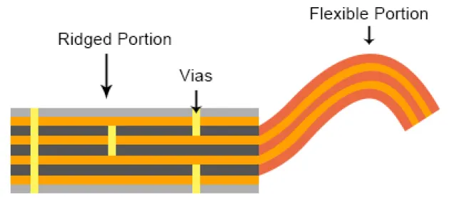
vi) Rigid-Flex PCB - Rigid-flex circuits combine the best of both worlds when it comes to the two most important overarching types of PCB boards. Flex-rigid boards consist of multiple layers of flexible PCBs attached to a number of rigid PCB layers.The combination of rigid and flexible boards into a single rigidflex board also allows for a more streamlined design, reducing the overall board size and package weight.

Other - Aluminum-Backed PCB, High-frequency PCB

Simulation Setup:

In this simulation, a PCB board, library files, and traces are imported to create the model. The model is first solved for conduction only without the components and then solved using the actual components with forced convection at last Joule heating phenomenon will be analysed.

• First import board layout *.bdf & *.ldf files in the Icepak. Filter the very small components which are not necessary in the simulation using the size filter with 8 mm as size.
  
  
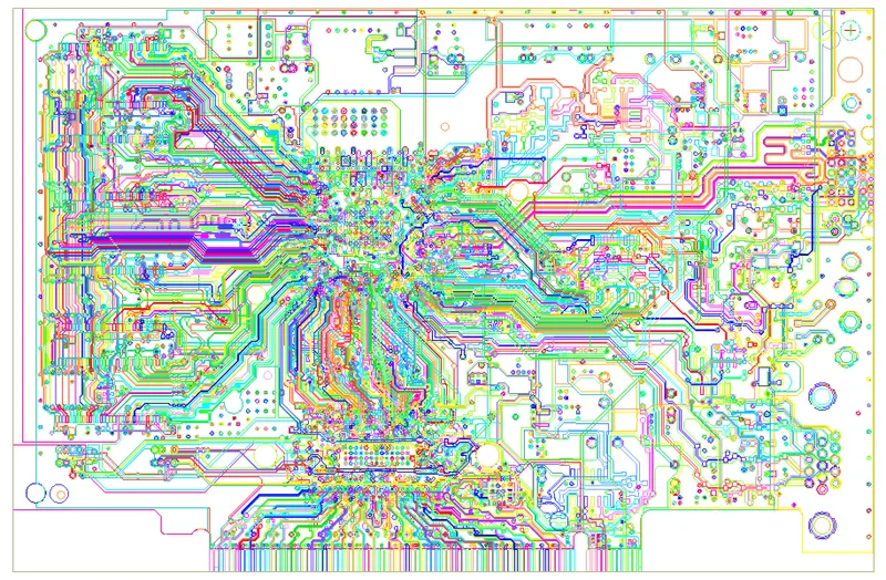
• Import ECAD file (*.anf) A1.anf inside ECAD Geometry section of 'Board'.
  
  

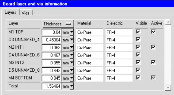
• Layer No.	Layer Thickness (mm)
  1	0.04
  2	0.45364
  3	0.062
  4	0.467
  5	0.055
  6	0.442
  7	0.045

  
  
  
  
• Specify Grid density by size (0.508 mm X 0.508 mm)
  
  
  
  

1] Conduction only model:

• Inactive all the components except "Board".
• Create wall B.C for cabinet in min_z and max_z direction.
• Assign a temperature B.C for the min_z side equal to 20 C and heat flux of 20000 W/m2 on min_z side.
• Disable flow and radiation option in the basic settings for simulation setup and use laminar flow option.
• Basic parameters: Flow & Radiation is off
• Set no. of iterations 500 and convergence criteria for energy to 1e-12.
• Temperature Linear solver: F cycle is selected and entered 1e-6 for both the Termination criterion and Residual reduction tolerance.
• Select Double for the solver precision.
  
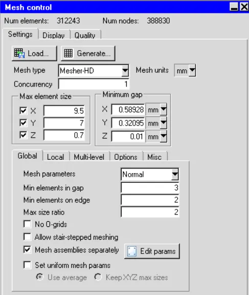
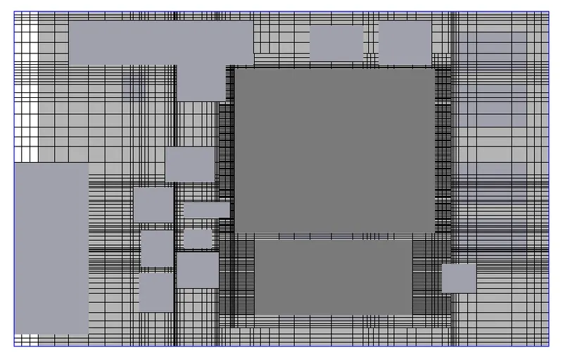
  Mesh Settings: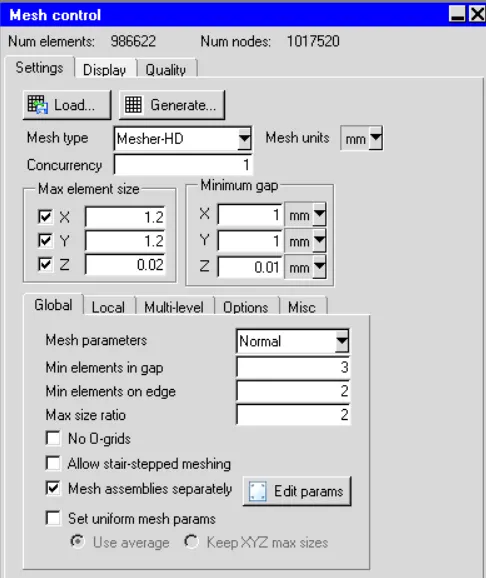
  
  
  
  

  Conduction Results:
  
  Residuals-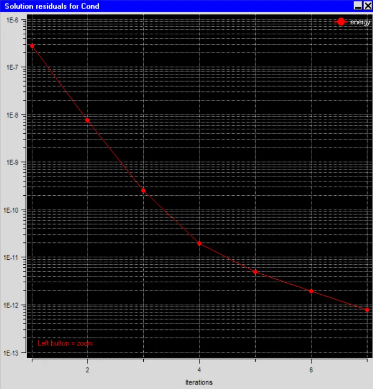
  
  
  
  

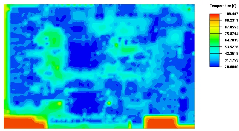
  Temperature Contour-

  
  

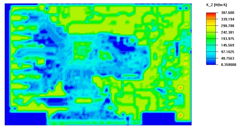
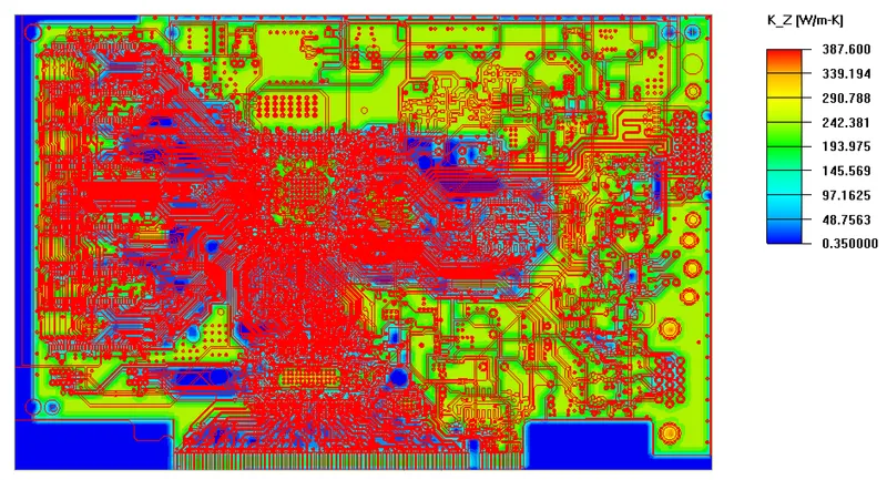
  Conductivity in K_Z direction (at the same location as of temp. contour)-

  

  
  
  
  

2] Force Convection Model:

• Activate all the components deactivated in the conduction simulation.
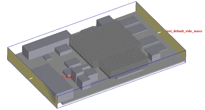
• Assign Wall B.C at all the sides of the cabinet except the min_x and max_x sides.
• Create an opening in the min_x and max_x sides of the cabinet and assign the velocity of -1.5 m/s to the max_x side.
  
  
• Basic parameters toggle on the Flow button. Keep and choose Turbulent and Zero equations for the flow regime
• set no of iterations 500 and convergence criteria for energy to 1e-12
• Temperature Linear solver: F cycle is selected for and entered 1e-6 for both the Termination criterion and Residual reduction tolerance.
• Select Double for the solver Precision.
• Enable Sequential solution of flow and energy equations.
  
  

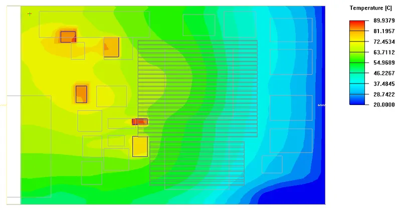
Convection Results: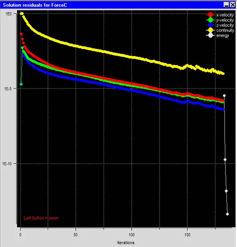

(Slider location at 0.075)

(Slider location at 0.075)

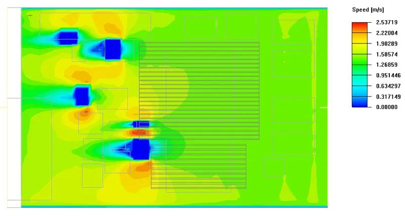
3] Joule/Trace Heating:

CB traces have electrical resistance, they heat up as current flows through them. Modelling this phenomenon will provide us with an accurate prediction of the temperature distribution in the PCB, which can be important, for example, in evaluating the performance of the cooling system.

• Create a solid trace of trace A3V3_2261.
• Create two sources connecting the trace and set current equal to 25 A for source_1 and voltage equal to 0 V for source_2.
• Use the same mesh setting as for the convection case.
• Set Resistivity, temperature coefficient (C), and reference temperature (Tref).
• The recommendation of the source objects pair for joule heating is the current-voltage pair or voltage-voltage pair.
• Use the Zero equation for the turbulent flow model.
• Set no. of iterations 500 and convergence criteria for energy to 1e-8 and Flow is 1e-4.
• Temperature Linear solver: F cycle is selected and entered 1e-6 for both the Termination criterion and Residual reduction tolerance.
• Choose BCGSTAB as the Stabilization criterion for both Temperature and Joule Heating Potential.
• Keep remaining settings as it is as in the case of the Convection Model.
  
  
  

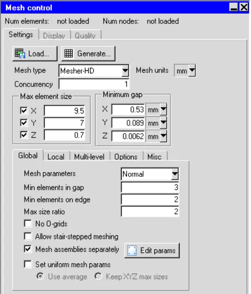
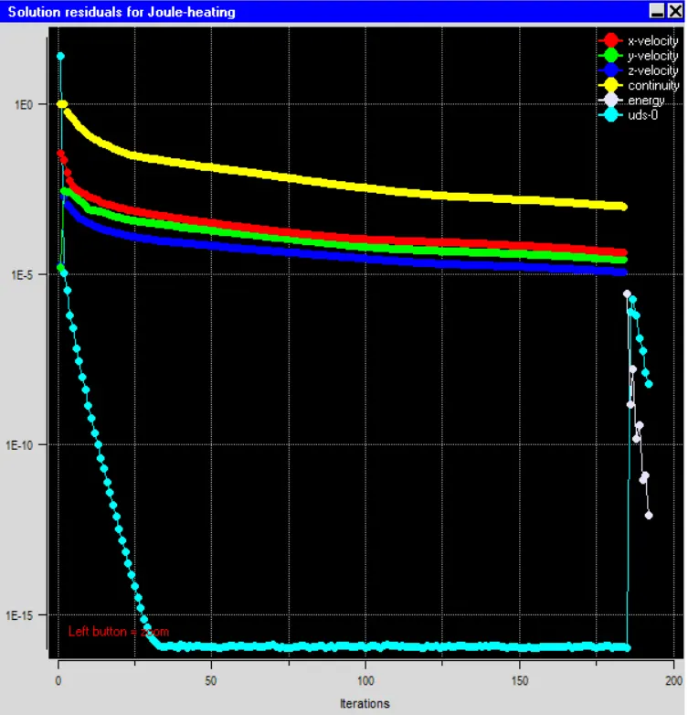
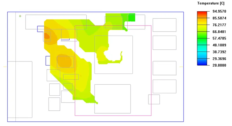
Joule Heating Results:

• 

  
  (Slider location at 0.075)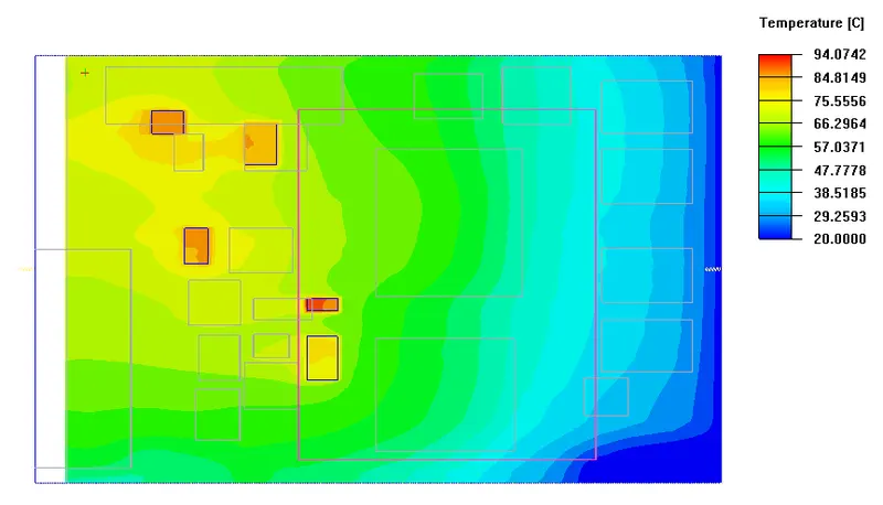
  

  (Slider location at 0.075)

  
  

Conclusion:

From the above results, we can see that the temperature is higher for the Joule heating than for the convention case alone. The temperature has raised from 89.9 C to 94.9 C due to Joule heating. Hence it is important to model the effect of Current flowing through PCB to accurately estimate the temperature. But here we considered only one trace, we need to model all other traces carrying current.