Simulating Cyclone separator with Discrete Phase Modelling
Simulating Cyclone separator with Discrete Phase Modelling
Introduction:
In this project, we are going to perform cyclone separator simulation with the Discrete Phase Modelling technique.
In addition to solving transport equations for the continuous phase the solver simulate a discrete second phase in a Lagrangian frame of reference. This second phase consists of spherical particles (which may be taken to represent droplets or bubbles) dispersed in the continuous phase. Solver computes the trajectories of these discrete phase entities, as well as heat and mass transfer to/from them. The coupling between the phases and its impact on both the discrete phase trajectories and the continuous phase flow can be included.
Cyclone Separator:
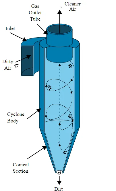
Cyclone separators are separation devices (dry scrubbers) that use the principle of inertia to remove particulate matter from flue gases.
A high speed rotating (air)flow is established within a cylindrical or conical container called a cyclone. Air flows in a spiral pattern, beginning at the top (wide end) of the cyclone and ending at the bottom (narrow) end before exiting the cyclone in a straight stream through the center of the cyclone and out the top. Larger (denser) particles in the rotating stream have too much inertia to follow the tight curve of the stream and strike the outside wall, falling then to the bottom of the cyclone where they can be removed. In a conical system, as the rotating flow moves towards the narrow end of the cyclone the rotational radius of the stream is reduced, separating smaller and smaller particles.
For large size granules, the separating rate can reach above 97%. The granule in smaller size or is more light, the more difficult to separate effectively.
There are varies proportions and styles of the cyclone separator, which generate different pressure losses. Usually, pressure loss of the cyclone separator is about 50~200mmAq.
Features Required:
High efficiency over a broad flow range
Flow-optimized design
Low-pressure drop resulting in energy savings
High safety during operation under pressure
Long-term corrosion protection
EMPIRICAL MODELS FOR THE PREDICTION OF CYCLONE EFFICIENCY
1] IOZIAAND LEITH MODEL
Iozia and Leith logistic model is a modified version of Barth model which is developed based on force balance. The model assumes that a particle carried by the vortex endures the influence of two forces: a centrifugal force, Z, and a flow resistance, W.
The addition made by Iozia and Leith on the original Barth model are the core length 'zc' and slope parameter 'beta'
expression which is derived based on the statistical analysis of experimental data of cyclone with D = 0.25 m.
Collection Efficiency = `eta_i = 1/(1 + (d_(pc)/bard_(p.i))^beta`
2] LI AND WANG MODEL
The Li and Wang model includes particle bounce or re-entrainment and turbulent diffusion at the cyclone wall. A two-dimensional analytical expression of particle distribution in the cyclone is obtained.
Li and Wang model was developed based on the following assumptions:
- The radial particle velocity and the radial concentration
profile are not constant, for uncollected particles within the
cyclones. - The tangential velocity is related to the radius of cyclone by `uR^n`.
Collection Efficiency = `n_i = 1 - exp(-lambda*theta_1)`
3] KOCH AND LICHT MODEL
Koch and Licht (1977) collection theory recognized the inherently turbulent nature of cyclones and the distribution of
gas residence times within the cyclone. Koch and Licht describe particle motion in the entry and collection regions
with the additional following assumptions:
• The tangential velocity of a particle is equal to the tangential velocity of the gas flow, i.e. there is no slip in the tangential
direction between the particle and the gas.
• The tangential velocity is related to the radius of cyclone by: uRn = constant.
Grade Efficiency = `eta_i = 1 - exp{-2[(G*tau_i*Q)/(D^3)*(n+1)]^(0.5/(n+1))}`
4] LAPPLE MODEL
Lapple model was developed based on force balance without considering the flow resistance. Lapple assumed that a particle entering the cyclone is evenly distributed across the inlet opening. The particle that travels from inlet half width to the wall in the cyclone is collected with 50% efficiency.
Efficiency of Collection of any size of the particle = `eta_i = 1/(1 + (d_(pc)/bard_(p.i))^2`
Simulation Setup:
Case 1:
The velocity of particle and Gas = 3m/sec
i) Particle size = 1um
ii) Particle size = 2um
iii) Particle size = 3um
iv) Particle size = 4um
v) Particle size = 5um
Case 2:
Size of particel = 5um
i) The velocity of particle and Gas = 1m/sec
ii) The velocity of particle and Gas = 2m/sec
iii) The velocity of particle and Gas = 3m/sec
iv) The velocity of particle and Gas = 4m/sec
v) The velocity of particle and Gas = 5m/sec
Boundary Condition:
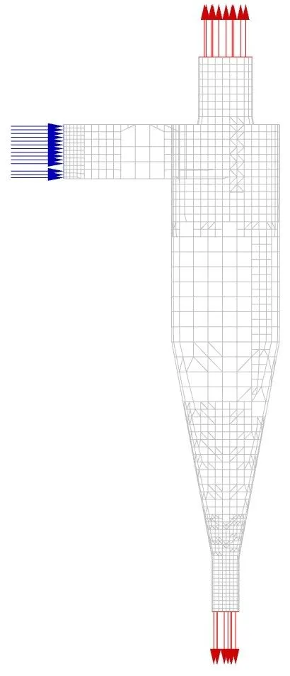
Inlet and Wall = Reflect
Outlet (Top) = Escape
Outlet (Bottom) = Trap
Mesh:
DPM Model Setup:
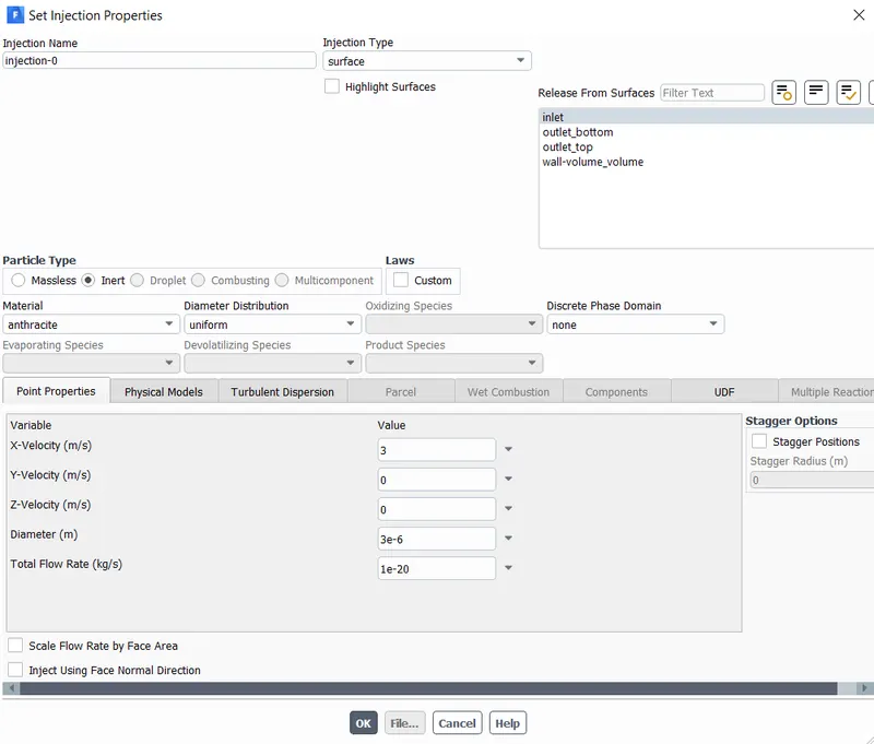
X-Velocity - Velocity of particles
Diameter - Diameter of particles tracked
Material - Material of particles
Injection type - Surface (Inlet of the cyclone)
Results:
Case 1:
The velocity of particle and Gas = 3m/sec
i) Particle size = 1um

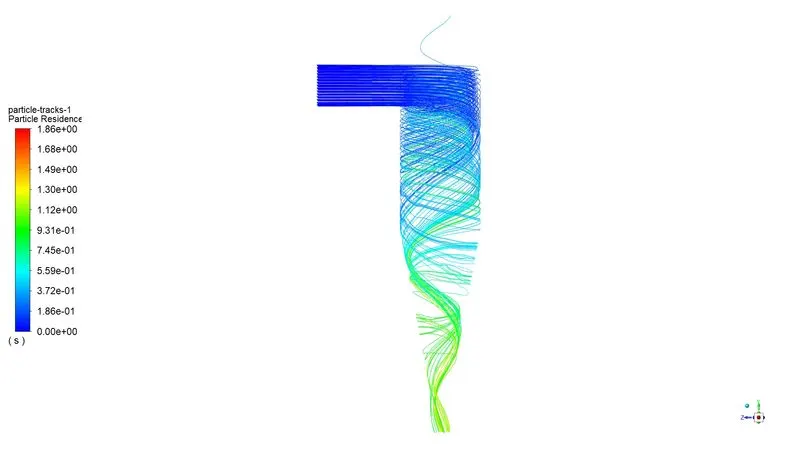
Separation Efficiency = No. of Particle Trapped / No. of particle Tracked
= 101/105 * 100 = 96.19%
ii) Particle size = 2um

Separation Efficiency = No. of Particle Trapped / No. of particle Tracked
= 100/105 * 100 = 95.2%
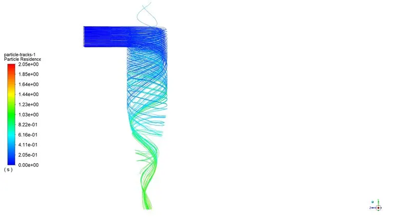
iii) Particle size = 3um

Separation Efficiency = No. of Particle Trapped / No. of particle Tracked
= 103/105 * 100 = 98%
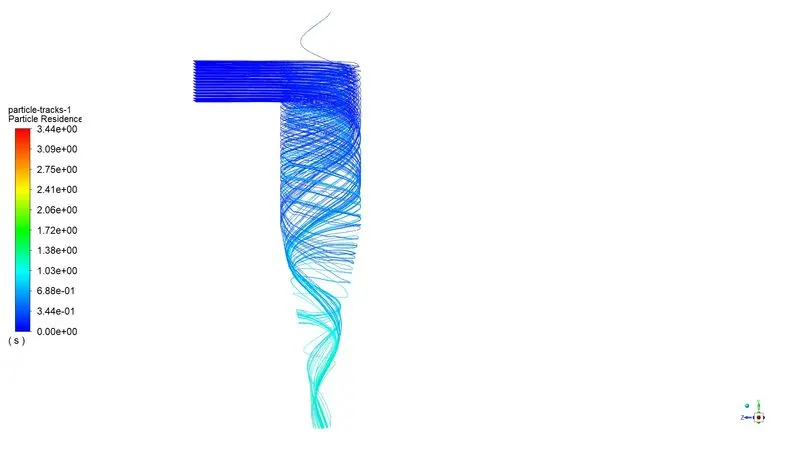
iv) Particle size = 4um

Separation Efficiency = No. of Particle Trapped / No. of particle Tracked
= 101/105 * 100 = 96.19%
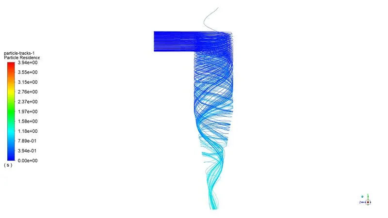
v) Particle size = 5um

Separation Efficiency = No. of Particle Trapped / No. of particle Tracked
= 101/105 * 100 = 96.19%
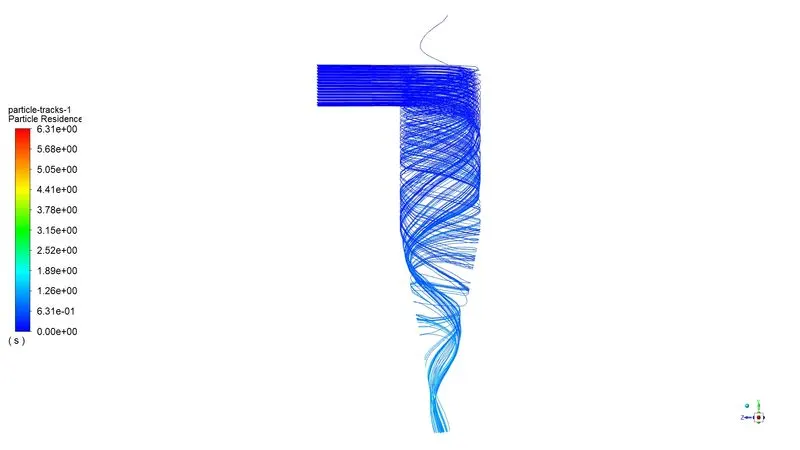
Case 2:
Size of particel = 5um
i) The velocity of particle and Gas = 1m/sec

Separation Efficiency = No. of Particle Trapped / No. of particle Tracked
= 98/105 * 100 = 93.33%
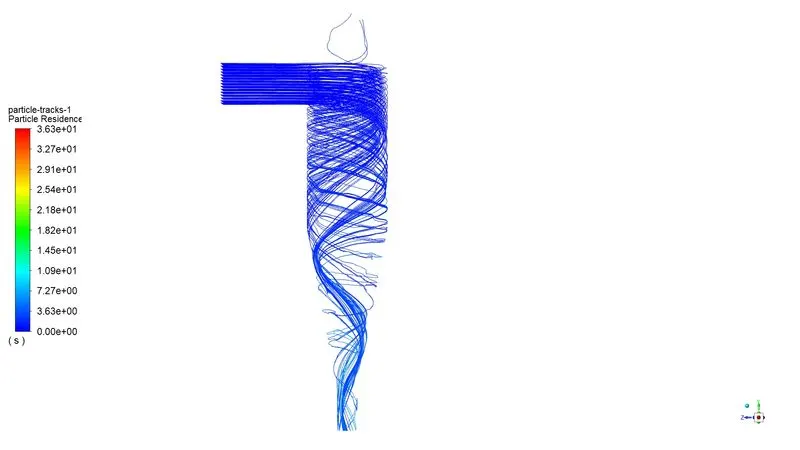
ii) The velocity of particle and Gas = 2m/sec

Separation Efficiency = No. of Particle Trapped / No. of particle Tracked
= 92/105 * 100 = 87.6%
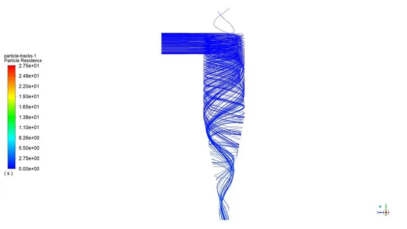
iii) The velocity of particle and Gas = 3m/sec

Separation Efficiency = No. of Particle Trapped / No. of particle Tracked
= 101/105 * 100 = 96.19%
iv) The velocity of particle and Gas = 4m/sec

Separation Efficiency = No. of Particle Trapped / No. of particle Tracked
= 103/105 * 100 = 98%
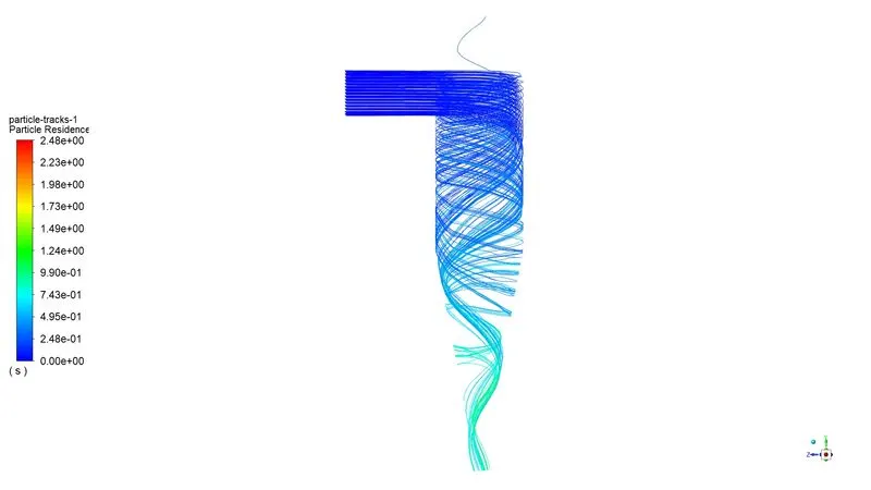
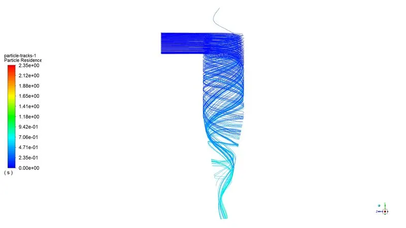
v) The velocity of particle and Gas = 5m/sec

Separation Efficiency = No. of Particle Trapped / No. of particle Tracked
= 103/105 * 100 = 98%
Conclusion:
From the above two analysis, it is observed that in case 1 when particle size is varied there is no major changes in the separation efficiency.
In case 2 when the velocity of particle and gas increases the separation efficiency is also increased.