Solving 2D heat conduction equation using an implicit and explicit method.
- Solving 2D Heat Conduction Equation Using an Implicit and Explicit Method.
- Use iterative solvers such as; Jacobi, Gauss-seidel, and Successive over-relaxation.
- Comparison of Fastest Steady-State Simulation and Fastest Transient Simulation.
List of Program -
1 ] Steady State Analysis
Implicit Scheme
i) Jacobi Method
ii) Gauss-Seidel Method
iii) SOR (Successive Over-relaxation) Method With Varying `omega`
2] Transient State Analysis
iv) Explicit Scheme
Implicit Scheme
v) Jacobi Method
vi) Gauss-Seidel Method
vii) SOR (Successive Over-relaxation) Method With Varying `omega`
viii) Explicit Scheme With `timeit(f)` Function
Implicit Scheme With timeit(f) Function
ix) Jacobi Method
x) Gauss-Seidel Method
xi) SOR (Successive Over-relaxation) Method With Varying `omega`
Implicit Scheme With Varying Time Step
xii) Gauss-Seidel *dt
xiii) SOR *dt
Introduction:
In this study, we are going to compare the fastest steady state and fastest transient simulation for 2-D heat conduction equation. We are going to look at the effect of `omega` in SOR method and effect of time_step on numerical schemes.
The conditions for the problem are as follows;
Top Boundary = `600 K`
Bottom Boundary = `900 K`
Left Boundary = `400 K`
Right Boundary = `800 K`
Length of domain in X and Y , `L=1`
Initial Temperature = `300 K`
We are going to implement the Implicit method on steady state analysis.
For transient case we will implement both Implicit and Explicit scheme.
In implicit scheme we use iterative solvers such as,
1. Jacobi
2. Gauss-seidel
3. Successive over-relaxation
Absolute error criteria = `1e-4`
1 ] Steady State Analysis:
Implicit Scheme
2-D Heat Conduction Equation,
`(del^2T)/(delx^2) + (delT^2)/(dely^2) = 0`
Discretization of the governing equation,
`Tp = 1/k*(Tl + Tr)/(Deltax^2) + 1/k*(Tt + Tb)/(Deltay^2)`
`l,r,t,b` represents location of node corresponding to node `p`. (Left, right, top and bottom)
i) Jacobi Method
Main Program:
clear; close all; clc

%{
Steady State (Implicit) Heat Conduction Using Jacobi Method
d2T/Dx2 + D2t/Dy2 = 0
%}
L = 1;      % Length of domain in X and Y
nx = 10;    % Nodes in X
ny = 10;    % Nodes in Y
dx = L/(nx-1);
dy = L/(ny-1);
k = (2*(dx^2 + dy^2))/(dx^2*dy^2);
x = linspace(0,L,nx);
y = linspace(0,L,ny);
T = 300*ones(nx,ny); % Initial Temperature
% Boundary Conditions
T(1,2:ny-1)= 600;
T(nx,2:ny-1)= 900;
T(2:nx-1,1)= 400;
T(2:nx-1,ny)= 800;
T(1,1)= 500;
T(1,ny)= 700;
T(nx,1)= 650;
T(nx,ny)= 850;
Told = T;
tol = 1e-4;
error = 1e4;
iterative_solver = 1;

if iterative_solver == 1
    iter = 1;
    while (error > tol)
        for i = 2:nx-1
            for j = 2:ny-1
                T(i,j) = (1/k)*(Told(i-1,j) + Told(i+1,j))/dx^2 + (1/k)*(Told(i,j-1) + Told(i,j+1))/dy^2;
            end
        end
            error = max(max(abs(Told - T)));
            Told = T;
            iter = iter + 1;
    end
end

heading  =  "Steady-State : Jacobi : Iterations = "+iter;
[X,Y] = meshgrid(x,y);
contourf(X,Y,Told, 10, 'ShowText','on')
set(gca, 'YDIR', 'reverse')
title(heading)
xlabel('x')
ylabel('y')
set(gca,'FontSize',12)
Output:
ii) Gauss-Seidel Method
Main Program:
clear; close all; clc

%{
Steady State (Implicit) Heat Conduction Using Gauss-Seidel Method
d2T/Dx2 + D2t/Dy2 = 0
%}
L = 1;        % Length of domain in X and Y
nx = 10;      % Nodes in X
ny = 10;      % Nodes in Y
dx = L/(nx-1);
dy = L/(ny-1);
k = (2*(dx^2 + dy^2))/(dx^2*dy^2);
x = linspace(0,L,nx);
y = linspace(0,L,ny);
T = 300*ones(nx,ny); % Initial Temperature
% Boundary Conditions
T(1,2:ny-1)= 600;
T(nx,2:ny-1)= 900;
T(2:nx-1,1)= 400;
T(2:nx-1,ny)= 800;
T(1,1)= 500;
T(1,ny)= 700;
T(nx,1)= 650;
T(nx,ny)= 850;
Told = T;
tol = 1e-4;
error = 1e4;
iterative_solver = 1;

if iterative_solver == 1
    iter = 1;
    while (error > tol)
        for i = 2:nx-1
            for j = 2:ny-1
                T(i,j) = (1/k)*(T(i-1,j) + Told(i+1,j))/dx^2 + (1/k)*(T(i,j-1) + Told(i,j+1))/dy^2;
            end
        end
            error = max(max(abs(Told - T)));
            Told = T;
            iter = iter + 1;
    end
end

heading  =  "Steady-State : G-Seidel : Iterations = "+iter;
[X,Y] = meshgrid(x,y);
contourf(X,Y,Told, 10, 'ShowText','on')
set(gca, 'YDIR', 'reverse')
title(heading)
xlabel('x')
ylabel('y')
set(gca,'FontSize',12)
Output:
iii) SOR Method
Main Program:
clear; close all; clc

%{
Steady State (Implicit) Heat Conduction Using SOR Method
d2T/Dx2 + D2t/Dy2 = 0
%}
L = 1;
nx = 10;
ny = 10;
dx = L/(nx-1);
dy = L/(ny-1);
k = (2*(dx^2 + dy^2))/(dx^2*dy^2);
x = linspace(0,L,nx);
y = linspace(0,L,ny);
T = 300*ones(nx,ny); % Initial Temperature
% Boundary Conditions
T(1,2:ny-1)= 600;
T(nx,2:ny-1)= 900;
T(2:nx-1,1)= 400;
T(2:nx-1,ny)= 800;
T(1,1)= 500;
T(1,ny)= 700;
T(nx,1)= 650;
T(nx,ny)= 850;
Told = T;
Tinitial = T;
tol = 1e-4;
relax_factor = [ 0.8 1 1.3 1.5 1.7 1.99];

for q = 1:length(relax_factor)
    w = relax_factor(q);
    Told = Tinitial;
    error = 1e4;
    iter = 1;
    while (error > tol)
        for i = 2:nx-1
            for j = 2:ny-1
                T(i,j) = (1-w)*Told(i,j) + w*((1/k)*(T(i-1,j) + Told(i+1,j))/dx^2 + (1/k)*(T(i,j-1) + Told(i,j+1))/dy^2);
            end
        end
            error = max(max(abs(Told - T)));
            Told = T;
            iter = iter + 1;
    end
     heading= "SOR : Iterations = "+iter+" : Relax-Factor = " +w;
     subplot(2,3,q)
    [X,Y] = meshgrid(x,y);
    contourf(X,Y,Told, 10, 'ShowText','on')
    set(gca, 'YDIR', 'reverse')
    title(heading)
    xlabel('x')
    ylabel('y')
    set(gca,'FontSize',10)
end
Output:
2 ] Transient State Analysis:
2-D Heat Conduction Equation,
`(del^2T)/(delt^2) = alpha*((del^2T)/(delx^2) + (del^2T)/(dely^2) )`
Discretization of the governing equation for explicit scheme,
`T^(n+1)p = T^np + k1*(Tl - 2Tp + Tr)^n + k2*(Tt - 2Tp +Tb)^n`
Time Step Size dt = 0.002
Time t = 20
alpha (a) = 1.4
Number of time steps nt = t/dt
CFL Number = `a*(Deltat)/(Deltax^2) = 0.23`
Note: In the following programs we have used 'While Loop' instead of moving forward according to number of time_steps since, we need to compare steady state simulation with transient state simulation. So, we have kept an error limit of 1e-4 as we have done in our previous steady state simulation.
iv) Explicit Scheme
Main Program:
clear; close all; clc

%{
Transient Explicit Heat Conduction
dT/dt = a*(d2T/Dx2 + D2t/Dy2)
%}

L = 1;
nx = 10;
ny = 10;
dx = L/(nx-1);
dy = L/(ny-1);
a = 1.4;
x = linspace(0,L,nx);
y = linspace(0,L,ny);
T = 300*ones(nx,ny); % Initial Temperature
% Boundary Conditions
T(1,2:ny-1)= 600;
T(nx,2:ny-1)= 900;
T(2:nx-1,1)= 400;
T(2:nx-1,ny)= 800;
T(1,1)= 500;
T(1,ny)= 700;
T(nx,1)= 650;
T(nx,ny)= 850;
Told = T;% Temperature is previous time step
dt = 0.002;  % Time Step Size
k1 = (a*dt)/dx^2;
k2 = (a*dt)/dy^2;
tol = 1e-4;
error = 1e4;
iter = 1;

while (error > tol)
    for i = 2:nx-1
        for j = 2:ny-1
            T(i,j) = Told(i,j) + k1*(Told(i-1,j) - 2*Told(i,j) + Told(i+1,j)) + k2*(Told(i,j-1) - 2*Told(i,j) + Told(i,j+1));
        end
    end
    error = max(max(abs(Told - T)));
    Told = T;
    iter = iter + 1;
end

heading = "Transient : Explicit Method : Iterations = "+ iter;
[X,Y] = meshgrid(x,y);
contourf(X,Y,Told, 10, 'ShowText','on')
set(gca, 'YDIR', 'reverse')
title(heading)
xlabel('x')
ylabel('y')
set(gca,'FontSize',12)
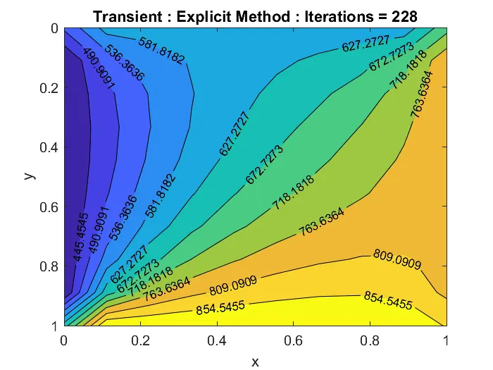
Output:
Implicit Scheme:
v) Jacobi Method
Main Program:
clear; close all; clc

%{
Transient Implicit Heat Conduction using Jacobi Method
dT/dt = a*(d2T/Dx2 + D2t/Dy2)
%}

L = 1;
nx = 10;
ny = 10;
dx = L/(nx-1);
dy = L/(ny-1);
a = 1.4;
x = linspace(0,L,nx);
y = linspace(0,L,ny);
T = 300*ones(nx,ny); % Initial Temperature
% Boundary Conditions
T(1,2:ny-1)= 600;
T(nx,2:ny-1)= 900;
T(2:nx-1,1)= 400;
T(2:nx-1,ny)= 800;
T(1,1)= 500;
T(1,ny)= 700;
T(nx,1)= 650;
T(nx,ny)= 850;
Told = T;     % T Guess
Tp = T;      % Temperature is previous time step
dt = 0.002;  % Time Step Size
k1 = (a*dt)/dx^2;
k2 = (a*dt)/dy^2;
tol = 1e-4;
error = 1e4;
iter = 1;

while (error > tol)
    for i = 2:nx-1
        for j = 2:ny-1
            Term1=1/(1+2*k1+2*k2);
            Term2 = k1*Term1;
            Term3 = k2*Term1;
            H = Told(i-1,j)+Told(i+1,j);
            V = Told(i,j-1)+Told(i,j+1);
            T(i,j) = (Tp(i,j)*Term1) + (H*Term2) + (V*Term3 );
         end
    end
    error = max(max(abs(Told - T)));
    Told = T;
    iter = iter + 1;
    Tp = T;
end

heading= "Transient : Jacobi Method : Iterations = "+iter;
[X,Y] = meshgrid(x,y);
contourf(X,Y,Told, 10, 'ShowText','on')
set(gca, 'YDIR', 'reverse') %matrix is reverse
title(heading)
xlabel('x')
ylabel('y')
set(gca,'FontSize',12)
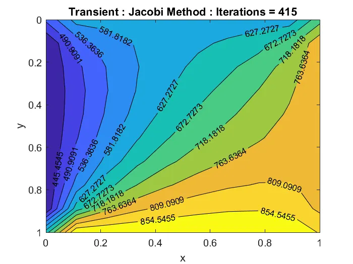
Output:
vi) Gauss-Seidel
Main Program:
clear; close all; clc

%{
Transient Implicit Heat Conduction Using Gauss-Seidel Method
dT/dt = a*(d2T/Dx2 + D2t/Dy2)
%}

L = 1;
nx = 10;
ny = 10;
dx = L/(nx-1);
dy = L/(ny-1);
a = 1.4;
x = linspace(0,L,nx);
y = linspace(0,L,ny);
T = 300*ones(nx,ny); % Initial Temperature
% Boundary Conditions
T(1,2:ny-1)= 600;
T(nx,2:ny-1)= 900;
T(2:nx-1,1)= 400;
T(2:nx-1,ny)= 800;
T(1,1)= 500;
T(1,ny)= 700;
T(nx,1)= 650;
T(nx,ny)= 850;
Told = T;     % T Guess
Tp = T;      % Temperature is previous time step
dt = 0.002;  % Time Step Size
k1 = (a*dt)/dx^2;
k2 = (a*dt)/dy^2;
tol = 1e-4;
error = 1e4;
iter  = 1;

while (error > tol)
            for i = 2:nx-1
                for j = 2:ny-1
                    Term1=1/(1+2*k1+2*k2);
                    Term2 = k1*Term1;
                    Term3 = k2*Term1;
                    H = T(i-1,j)+Told(i+1,j);
                    V = T(i,j-1)+Told(i,j+1);
                    T(i,j) = (Tp(i,j)*Term1) + (H*Term2) + (V*Term3 );
                 end
            end
            error = max(max(abs(Told - T)));
            Told = T;
            iter = iter + 1;
            Tp = T;
end

heading= "Transient : G-Seidel Method : Iterations = "+iter;
[X,Y] = meshgrid(x,y);
contourf(X,Y,Told, 10, 'ShowText','on')
set(gca, 'YDIR', 'reverse')
title(heading)
xlabel('x')
ylabel('y')
set(gca,'FontSize',12)
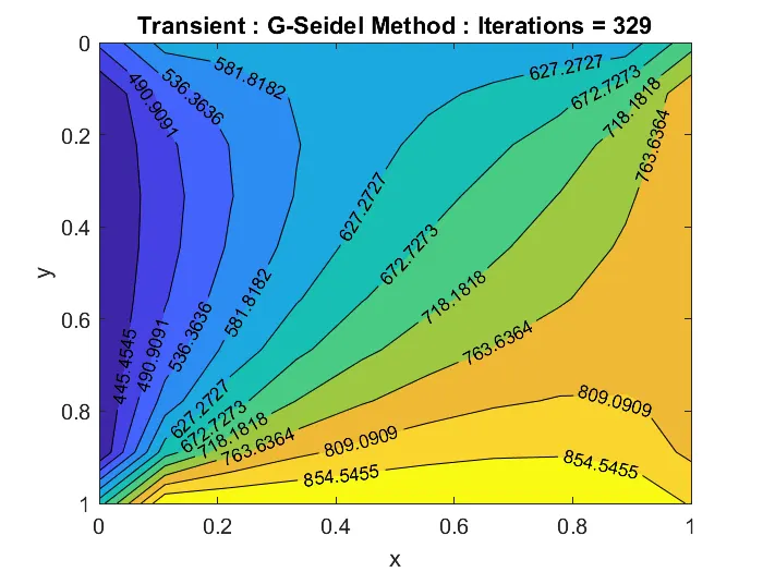
Output:
vii) SOR Method
Main Program:
clear; close all; clc

%{
Transient Implicit Heat Conduction Using SOR Method
dT/dt = a*(d2T/Dx2 + D2t/Dy2)
%}

L = 1;
nx = 10;
ny = 10;
dx = L/(nx-1);
dy = L/(ny-1);
a = 1.4;
x = linspace(0,L,nx);
y = linspace(0,L,ny);
T = 300*ones(nx,ny); % Initial Temperature
% Boundary Conditions
T(1,2:ny-1)= 600;
T(nx,2:ny-1)= 900;
T(2:nx-1,1)= 400;
T(2:nx-1,ny)= 800;
T(1,1)= 500;
T(1,ny)= 700;
T(nx,1)= 650;
T(nx,ny)= 850;
Told = T;     % T Guess
Tp = T;
Tinitial = T;
dt = 0.002;  % Time Step Size
k1 = (a*dt)/dx^2;
k2 = (a*dt)/dy^2;
tol = 1e-4;
error = 1e4;
relax_factor = [ 0.8 1 1.3 2 4.2 4.3];
iter = 1;

for q = 1:length(relax_factor)
    w = relax_factor(q);
    Told = Tinitial;
    Tp = Tinitial;
    error = 1e4;
    iter = 1;
    while (error > tol)
        for i = 2:nx-1
            for j = 2:ny-1
                Term1=1/(1+2*k1+2*k2);
                Term2 = k1*Term1;
                Term3 = k2*Term1;
                H = T(i-1,j)+Told(i+1,j);
                V = T(i,j-1)+Told(i,j+1);
                T(i,j) = (1-w)*Told(i,j) + w*((Tp(i,j)*Term1) + (H*Term2) + (V*Term3 ));
             end
        end
        error = max(max(abs(Told - T)));
        Told = T;
        iter = iter + 1;
        Tp = T;
    end
     heading= "SOR : Iterations = "+iter+" : Relax-Factor = " +w;
     subplot(2,3,q)
    [X,Y] = meshgrid(x,y);
    contourf(X,Y,Told, 10, 'ShowText','on')
    set(gca, 'YDIR', 'reverse')
    title(heading)
    xlabel('x')
    ylabel('y')
    set(gca,'FontSize',10)
end
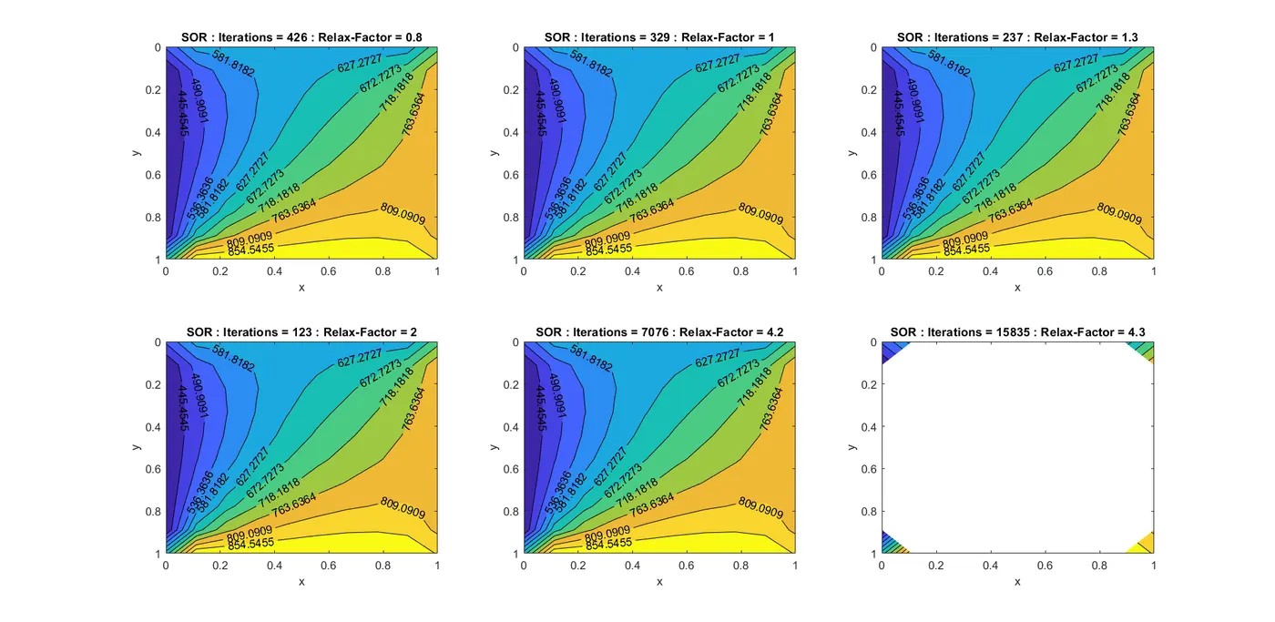
Output:
Note: In the following programs we have used 'timeit(f)' function to measure time take to execute the program. The Output of the program has been mentioned as an avarage time by running the program several times.
xiii) Explicit Scheme:
Function: get_time_explicit
function Texp = get_time_explicit()

L = 1;                  a = 1.4;
nx = 10;                ny = 10;
dx = L/(nx-1);          dy = L/(ny-1);
T = 300*ones(nx,ny);    % Initial Temperature
% Boundary Conditions %
T(1,2:ny-1)= 600;       T(nx,2:ny-1)= 900;
T(2:nx-1,1)= 400;       T(2:nx-1,ny)= 800;
T(1,1)= 500;            T(1,ny)= 700;
T(nx,1)= 650;           T(nx,ny)= 850;
Told = T;               % Temperature is previous time step
dt = 0.002;             % Time Step Size
t = 20;                 % Time
nt = t/dt;              % Number of time steps
k1 = (a*dt)/dx^2;       k2 = (a*dt)/dy^2;

for clock = 1:nt
    for i = 2:nx-1
        for j = 2:ny-1
            T(i,j) = Told(i,j) + k1*(Told(i-1,j) - 2*Told(i,j) + Told(i+1,j)) + k2*(Told(i,j-1) - 2*Told(i,j) + Told(i,j+1));
        end
    end
        Told = T;
end
Texp = T;
end
Main Program:
clear; close all; clc

%{
Transient Explicit Heat Conduction
dT/dt = a*(d2T/Dx2 + D2t/Dy2)
%}

solve = @()get_time_explicit()
Time_Explicit = timeit(solve)
Output: Average_Time = 0.0069 sec
Implicit Scheme:
xi) Jacobi Method
Function: get_time_jacobi
function Tj = get_time_jacobi()

L = 1;                  a = 1.4;
nx = 10;                ny = 10;
dx = L/(nx-1);          dy = L/(ny-1);
T = 300*ones(nx,ny);    % Initial Temperature
% Boundary Conditions %
T(1,2:ny-1)= 600;       T(nx,2:ny-1)= 900;
T(2:nx-1,1)= 400;       T(2:nx-1,ny)= 800;
T(1,1)= 500;            T(1,ny)= 700;
T(nx,1)= 650;           T(nx,ny)= 850;
Told = T;               Tp = T;
dt = 0.002;             % Time Step Size
t = 20;                 % Time
nt = t/dt;              % Number of time steps
k1 = (a*dt)/dx^2;       k2 = (a*dt)/dy^2;
tol = 1e-4;

for clock = 1:nt
    error = 1e4;
        while (error > tol)
            for i = 2:nx-1
                for j = 2:ny-1
                    Term1=1/(1+2*k1+2*k2);
                    Term2 = k1*Term1;
                    Term3 = k2*Term1;
                    H = Told(i-1,j)+Told(i+1,j);
                    V = Told(i,j-1)+Told(i,j+1);
                    T(i,j) = (Tp(i,j)*Term1) + (H*Term2) + (V*Term3 );
                 end
            end
            error = max(max(abs(Told - T)));
            Told = T;
        end
         Tp = T;
end
    Tj = T;
end
Main Program:
clear; close all; clc

%{
Transient Implicit Heat Conduction using Jacobi Method
dT/dt = a*(d2T/Dx2 + D2t/Dy2)
%}

solve = @()get_time_jacobi()
Time_Jacobi = timeit(solve)
Output: Average_Time = 0.0135 sec
x) Gauss-Seidel Method
Function: get_time_gausseidel
function Tg = get_time_gausseidel()

L = 1;                  a = 1.4;
nx = 10;                ny = 10;
dx = L/(nx-1);          dy = L/(ny-1);
T = 300*ones(nx,ny);    % Initial Temperature
% Boundary Conditions %
T(1,2:ny-1)= 600;       T(nx,2:ny-1)= 900;
T(2:nx-1,1)= 400;       T(2:nx-1,ny)= 800;
T(1,1)= 500;            T(1,ny)= 700;
T(nx,1)= 650;           T(nx,ny)= 850;
Told = T;               Tp = T;
dt = 0.002;             % Time Step Size
t = 20;                 % Time
nt = t/dt;              % Number of time steps
k1 = (a*dt)/dx^2;       k2 = (a*dt)/dy^2;
tol = 1e-4;

for clock = 1:nt
    error = 1e4;
        while (error > tol)
            for i = 2:nx-1
                for j = 2:ny-1
                    Term1=1/(1+2*k1+2*k2);
                    Term2 = k1*Term1;
                    Term3 = k2*Term1;
                    H = T(i-1,j)+Told(i+1,j);
                    V = T(i,j-1)+Told(i,j+1);
                    T(i,j) = (Tp(i,j)*Term1) + (H*Term2) + (V*Term3 );

                 end
            end
            error = max(max(abs(Told - T)));
            Told = T;
        end
         Tp = T;
end
Tg= T;
end
Main Program:
clear; close all; clc

%{
Transient Implicit Heat Conduction using Gauss-Seidel Method
dT/dt = a*(d2T/Dx2 + D2t/Dy2)
%}

solve = @()get_time_gausseidel()
Time_Gauss_Seidel = timeit(solve)
Output: Average_Time = 0.0129 sec
Xi) SOR Method
Function: get_time_sor
function Ts = get_time_sor(w)

L = 1;                  a = 1.4;
nx = 10;                ny = 10;
dx = L/(nx-1);          dy = L/(ny-1);
T = 300*ones(nx,ny);    % Initial Temperature
% Boundary Conditions %
T(1,2:ny-1)= 600;       T(nx,2:ny-1)= 900;
T(2:nx-1,1)= 400;       T(2:nx-1,ny)= 800;
T(1,1)= 500;            T(1,ny)= 700;
T(nx,1)= 650;           T(nx,ny)= 850;
Told = T;               Tp = T;
dt = 0.002;             % Time Step Size
t = 20;                 % Time
nt = t/dt;              % Number of time steps
k1 = (a*dt)/dx^2;       k2 = (a*dt)/dy^2;
tol = 1e-4;

for clock = 1:nt
    error = 1e4;
        while (error > tol)
            for i = 2:nx-1
                for j = 2:ny-1
                    Term1=1/(1+2*k1+2*k2);
                    Term2 = k1*Term1;
                    Term3 = k2*Term1;
                    H = T(i-1,j)+Told(i+1,j);
                    V = T(i,j-1)+Told(i,j+1);
                    T(i,j) = (1-w)*Told(i,j) + w*((Tp(i,j)*Term1) + (H*Term2) + (V*Term3 ));

                 end
            end
            error = max(max(abs(Told - T)));
            Told = T;
        end
         Tp = T;
end
Ts= T;
end
Main Program:
clear; close all; clc

%{
Transient Implicit Heat Conduction using SOR Method
dT/dt = a*(d2T/Dx2 + D2t/Dy2)
%}
Relax_Factor = [ 0.6 0.8 1 1.3 1.8 1.9 ];
for k = 1:length(Relax_Factor)
    w = Relax_Factor(k);
    solve = @()get_time_sor(w);
    Time_for_SOR = "Time_SOR for Relax_Factor = "+w+" is = "+timeit(solve)
end
Output:
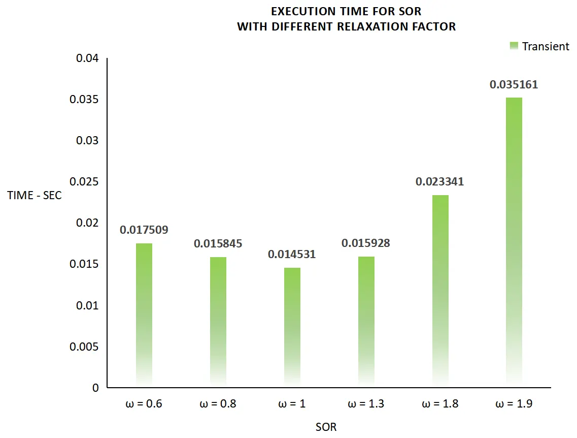
Time_SOR for Relax_Factor = 0.6 is = 0.017509 sec
Time_SOR for Relax_Factor = 0.8 is = 0.015845 sec
Time_SOR for Relax_Factor = 1 is = 0.014531 sec
Time_SOR for Relax_Factor = 1.3 is = 0.015928 sec
Time_SOR for Relax_Factor = 1.8 is = 0.023341 sec
Time_SOR for Relax_Factor = 1.9 is = 0.035161 sec
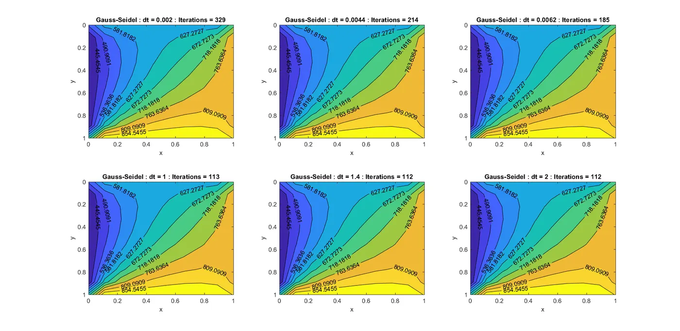
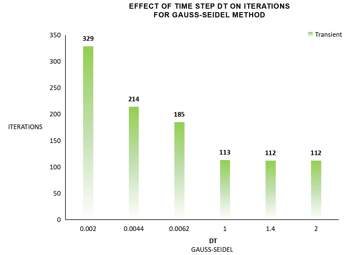
xii) Gauss-Seidel *dt: More faster simulation can be achived by increasing time step, therefore to compare its effect with steady state simulation, we have considered Gauss-Seidel method with varying time_step.
clear; close all; clc

%{
Transient Implicit Heat Conduction using Gauss-Seidel Method
dT/dt = a*(d2T/Dx2 + D2t/Dy2)
%}

L = 1;                  a = 1.4;
nx = 10;                ny = 10;
dx = L/(nx-1);          dy = L/(ny-1);
x = linspace(0,L,nx);   y = linspace(0,L,ny);
T = 300*ones(nx,ny);                            % Initial Temperature
% Boundary Conditions
T(1,2:ny-1)= 600;       T(nx,2:ny-1)= 900;
T(2:nx-1,1)= 400;       T(2:nx-1,ny)= 800;
T(1,1)= 500;            T(1,ny)= 700;
T(nx,1)= 650;           T(nx,ny)= 850;
Told = T;               Tinitial = T;           % T Guess
Tp = T;
time_step = [0.002  0.0044 0.0062 1 1.4 2];   % Time Step Size
tol = 1e-4;

for q  = 1:length(time_step)
    dt = time_step(q);
    k1 = (a*dt)/dx^2;
    k2 = (a*dt)/dy^2;
    Told = Tinitial;
    Tp   = Tinitial;
    error = 1e4;
    iter = 1;
        while (error > tol)
            for i = 2:nx-1
                for j = 2:ny-1
                    Term1=1/(1+2*k1+2*k2);
                    Term2 = k1*Term1;
                    Term3 = k2*Term1;
                    H = T(i-1,j)+Told(i+1,j);
                    V = T(i,j-1)+Told(i,j+1);
                    T(i,j) = (Tp(i,j)*Term1) + (H*Term2) + (V*Term3 );
                 end
            end
            error = max(max(abs(Told - T)));
            Told = T;
            Tp = T;
            iter = iter +1;
        end
            Tnew{q} = Told;
            heading  = "Gauss-Seidel : dt = " +dt+ " : Iterations = " +iter;
            subplot(2,3,q)
            [X,Y] = meshgrid(x,y);
            contourf(X,Y,Tnew{q}, 10, 'ShowText','on')
            set(gca, 'YDIR', 'reverse')
            title(heading)
            xlabel('x')
            ylabel('y')
            set(gca,'FontSize',10)
end
Output:
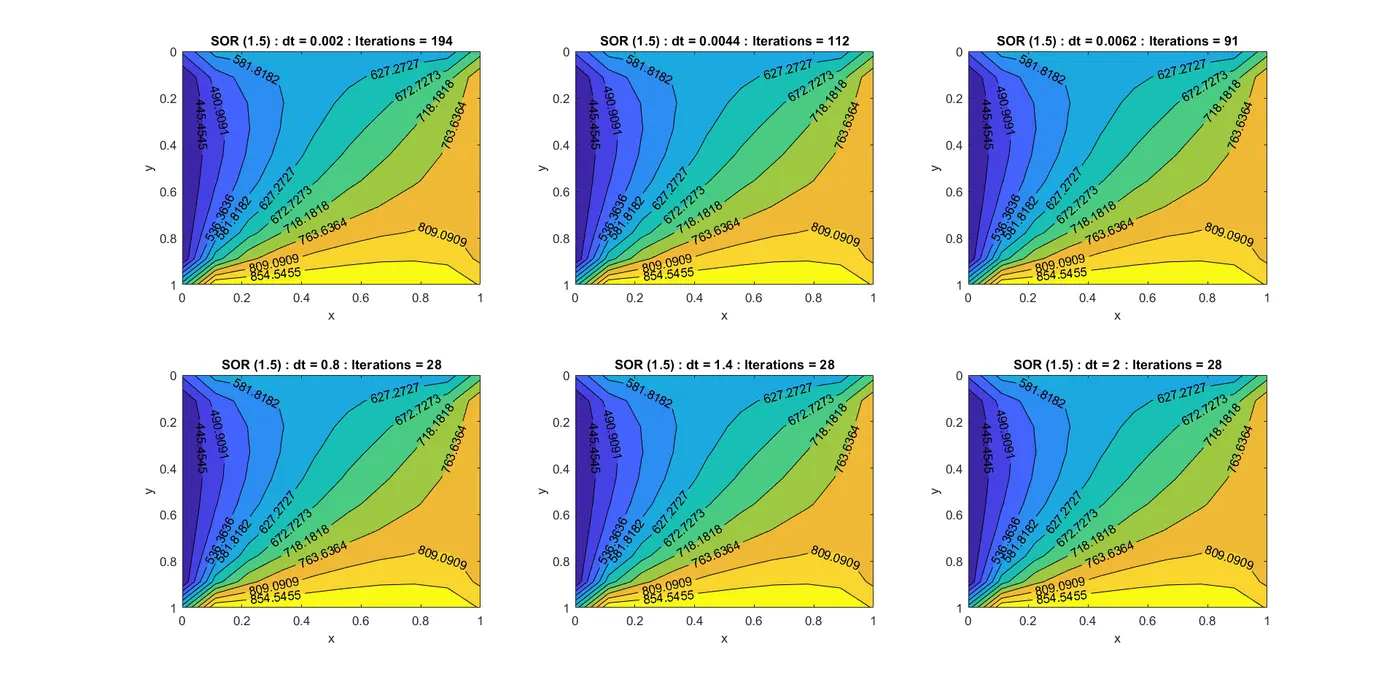
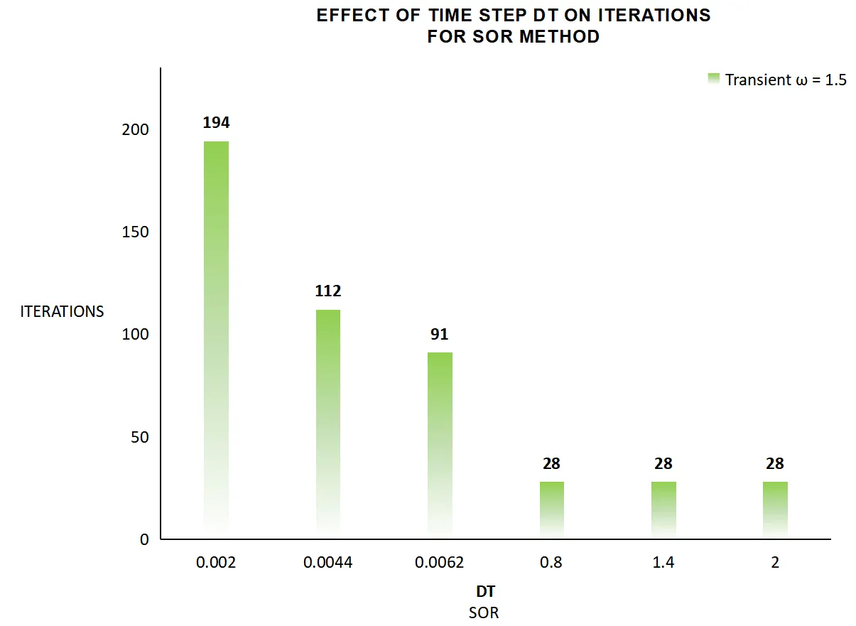
xiii) SOR *dt: Relaxation factor `omega = 1.5`. In this simualtion SOR method is tested for varying time_step. (Before taking fixed value of w = 1.5, I have checked the results for w = ...1.4,1.6...etc for varying time_step - dt and for steady state also relax_factor = 1.5 shows least iterations)
clear; close all; clc

%{
Transient Implicit Heat Conduction using SOR Method
dT/dt = a*(d2T/Dx2 + D2t/Dy2)
%}

%{
Before taking fixed value of w = 1.5, I have checked the
results for w = ...1.4,1.6...etc for varying time_step dt.
%}


L = 1;                  a = 1.4;
nx = 10;                ny = 10;
dx = L/(nx-1);          dy = L/(ny-1);
x = linspace(0,L,nx);   y = linspace(0,L,ny);
T = 300*ones(nx,ny);                            % Initial Temperature
% Boundary Conditions
T(1,2:ny-1)= 600;       T(nx,2:ny-1)= 900;
T(2:nx-1,1)= 400;       T(2:nx-1,ny)= 800;
T(1,1)= 500;            T(1,ny)= 700;
T(nx,1)= 650;           T(nx,ny)= 850;
Told = T;               Tinitial = T;           % T Guess
Tp = T;
time_step = [0.002  0.0044 0.0062 0.8 1.4 2];   % Time Step Size
tol = 1e-4;             w = 1.5;

for q  = 1:length(time_step)
    dt = time_step(q);
    k1 = (a*dt)/dx^2;
    k2 = (a*dt)/dy^2;
    Told = Tinitial;
    Tp   = Tinitial;
    error = 1e4;
    iter = 1;
        while (error > tol)
            for i = 2:nx-1
                for j = 2:ny-1
                    Term1=1/(1+2*k1+2*k2);
                    Term2 = k1*Term1;
                    Term3 = k2*Term1;
                    H = T(i-1,j)+Told(i+1,j);
                    V = T(i,j-1)+Told(i,j+1);
                    T(i,j) = (1-w)*Told(i,j) + w*((Tp(i,j)*Term1) + (H*Term2) + (V*Term3 ));
                 end
            end
            error = max(max(abs(Told - T)));
            Told = T;
            Tp = T;
            iter = iter +1;
        end
            Tnew{q} = Told;
            heading  = "SOR (1.5) : dt = " +dt+ " : Iterations = " +iter;
            subplot(2,3,q)
            [X,Y] = meshgrid(x,y);
            contourf(X,Y,Tnew{q}, 10, 'ShowText','on')
            set(gca, 'YDIR', 'reverse')
            title(heading)
            xlabel('x')
            ylabel('y')
            set(gca,'FontSize',10)
end
Output:
Results:
Note - Unless mentioned, all the following transient simulations are performed at time step dt = 0.002.
`1^(st)`
`2^(nd)`
`3^(rd)`
`4^(th)`
`5^(th)`
`6^(th)`
`7^(th)`
`8^(th)`
Discussion:
In this study we have compared the iterations/time taken by different solvers to compute a solution.
i) Steady State:
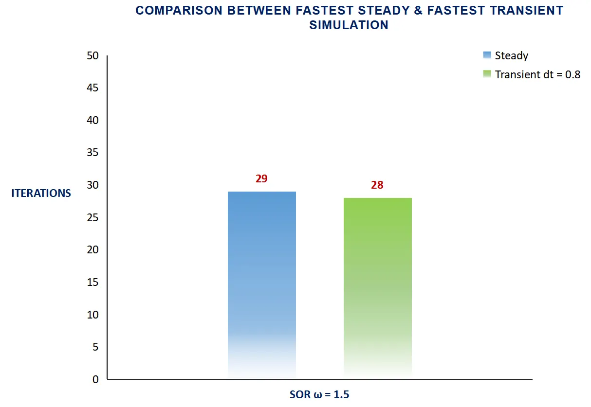
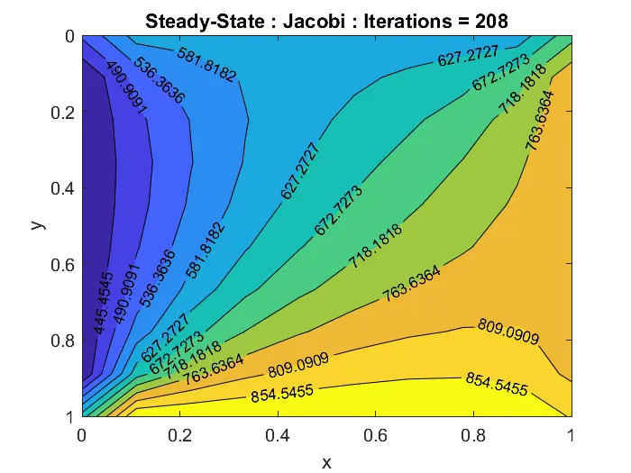
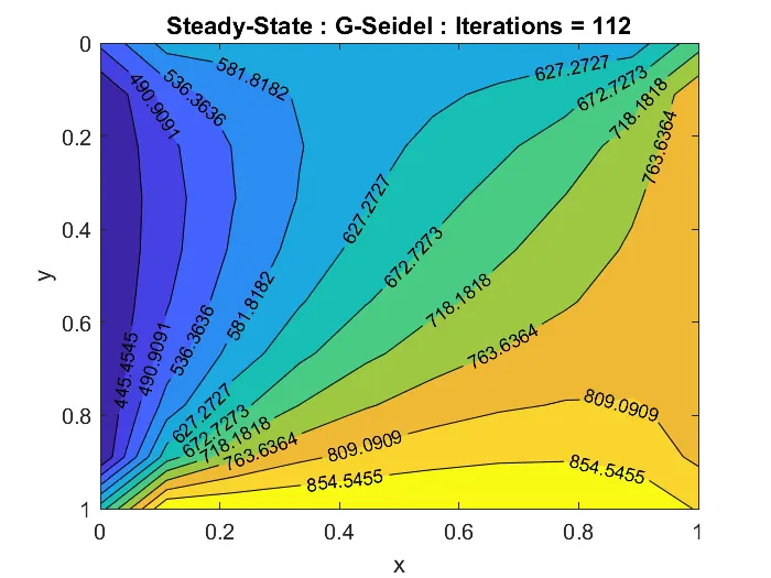
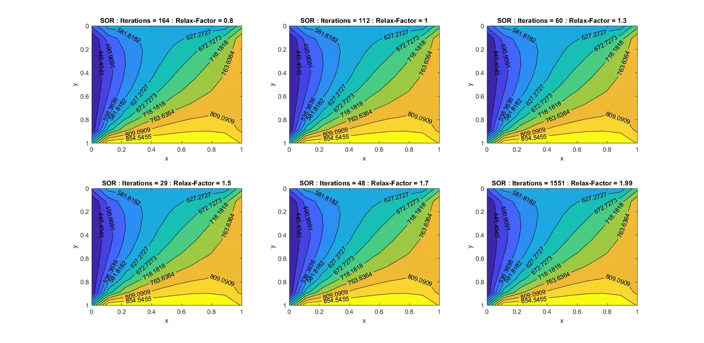
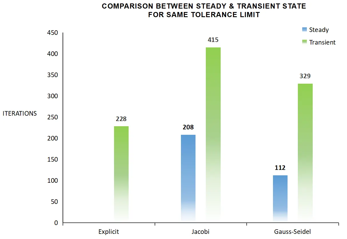
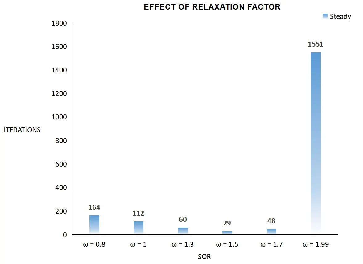
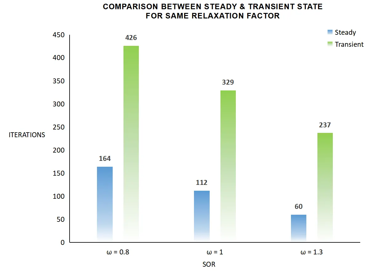
In the steady state simulation we have used implicit method to discretize the partial differential equation and then using point iterative method such as Jacobi, Gauss-Seidel, SOR we have solved the equation. From the 1st bar graph we can say that Gauss-Seidel is more faster than Jacobi. The number of iterations taken by SOR method depends upon the relaxation-factor (`omega`) and this effect of relaxation factor on number of iterations is shown in 2nd bar graph. The graph shows that as we increase the relaxation-factor the iterations taken by the solver decreases but after a particular value of relaxation-factor the number of iterations starts increasing, this is observed after `omega` > 1.5. If we compare SOR with previous two methods then SOR is more faster for the range of relaxation-factor between 1 < `omega` < 1.8 (approx). For `omega` < 1 & `omega` > 1.8 SOR method can be slower than Jacobi/Gauss-Seidel. Therefore final conclusion of fastest steady state simulation depends upon value of relaxation-factor. In our case, for `omega` = 1.5 SOR method takes least number of iterations i.e 29 iterations, hence this is our fastest steady state simulation.
ii) Transient State:
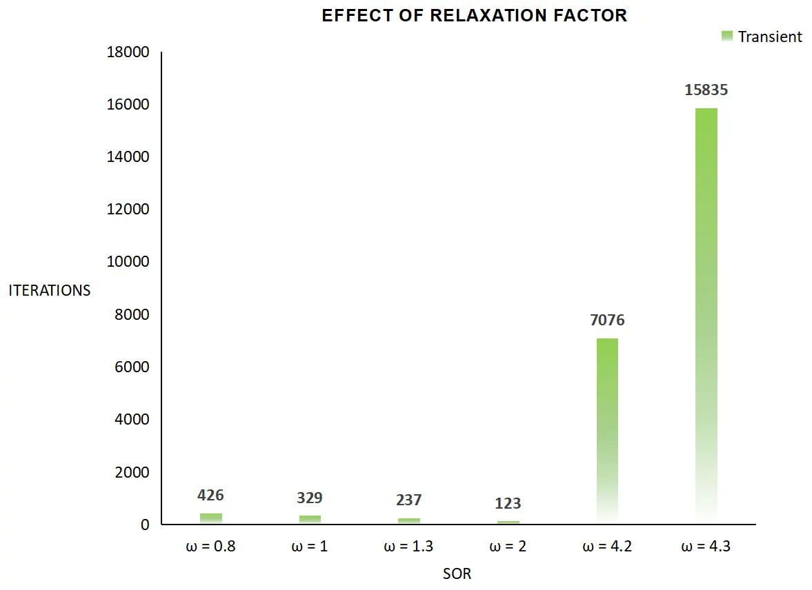
In transient simulation we have used both explicit and implicit scheme. The 1st bar graph shows that explicit scheme takes least number of iterations compared to Jacobi & Gauss-Seidel. The effect of relaxation-factor in SOR method is presented in 3rd bar graph. It’s effect is similar to what we have discussed in steady state simulation. Between the range 1 < `omega` < 2(approx) SOR method is more faster than Jacobi/Gauss-Seidel and for approx ~ 1.3 < `omega` < 2 the SOR method is faster than explicit method. Therefore, for `omega` = 2, SOR is the fastest transient method (123 iterations).
However, the number of iterations can be decreased if we increase the time_step ‘dt’. This effect of time_step on iterations is shown in 7th bar graph. Here we have considered only Gauss-Seidel method for varying time_step to compare it with steady state Gauss-Seidel. Similar effect can be seen on Jacobi method ( here we are excluding explicit scheme, since explicit scheme has very close limitation for CFL number, ex - 1 or 0.5). The 7th bar graph shows that as we increase the time_step, the number of iterations decreases and has reached to a constant value of 112 iterations after time_step 1.4. So, the least iterations (112) are observed at time_step dt = 1.4.
Taking range of time_steps we have also performed simulation on SOR method for relaxation-factor `omega` = 1.5. In the 8th bar graph similar trend is observed as in previous Gauss-Seidel case. In this case least iterations were calculated at time_step dt = 0.8 for 28 iterations. After this value of dt (0.8), the number of iterations remains constant.
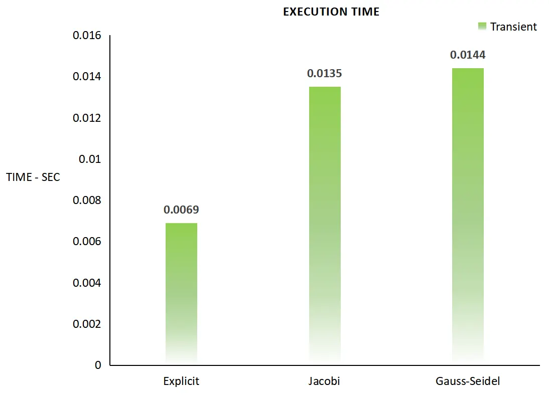
Using 'timeit' function: We have also used ‘timeit(f)’ function to measure execution time of program for transient state simulation results of which are mentioned in 5th & 6th bar graph. Form the 5th bar graph, the explicit scheme is faster than implicit scheme (Jacobi/Gauss-Seidel). The 6th bar graph shows execution time for SOR method with varying relaxation-factor. The effect of relaxation-factor on execution time is similar to our previous two cases (steady/transient) where we have focused on number of iterations taken by a solver. But in this case the execution time for SOR method is more than Jacobi and Gauss-Seidel method for approximately all the values of relaxation-factor. This trend decreases as we increase relaxation-factor from 0 < `omega` < 1 and then the trend increases as we increase the relaxation-factor `omega` > 1. If we consider ‘timeit(f)’ function for measurement of fastest transient simulation then explicit scheme is the fastest. The above program was ran on Matlab R2018a with serial processing, however if the simulation/scheme/method which we have discussed were ran with parallel processing then the results would be very different from the current study. Therefore, for comparison of fastest steady state and fastest transient simulation we will consider cases with number of iterations taken by the solver to reach the given tolerance limit 1e-4.
Conclusion:
From the above results and discussion, we can conclude that our fastest steady-state simulation ran for 29 iterations with SOR solver having relaxation-factor equal to 1.5. The fastest transient simulation ran for 28 iterations with SOR solver having relaxation-factor equal to 1.5 and time_step(minimum) size equal to 0.8. Hence, transient simulation is one iteration ahead but the number of iteration for the steady and transient state is quite the same and this has been achieved by proper selection of relaxation-factor and time_step. However, the use of larger time_step in transient simulation is not always recommended since in transient simulation at each time step we need accurate results and effects produced in the simulation.