Conjugate Heat Transfer Analysis on a graphics card.

Conjugate Heat Transfer Analysis on a graphics card

Introduction:

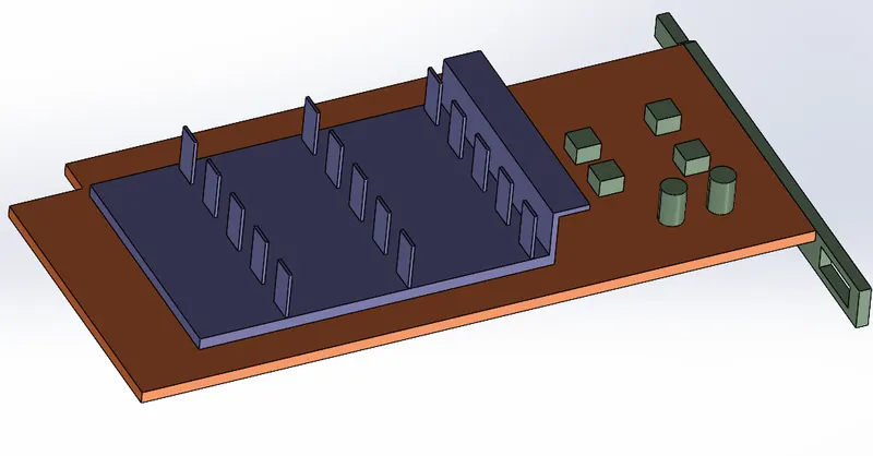
In this analysis, we are going to perform a conjugate heat transfer simulation on the graphic card and determine the heat transfer coefficient for the fluid-solid interface of the processor. Computer processors are designed to run at high temperatures and it's completely normal for a CPU to heat up and to actually get very warm. In fact, temperatures of over 200 degrees Fahrenheit are frequently acceptable. As electricity passes through the CPU or gets blocked inside, it gets turned into heat energy. To find out the heat transfer coefficient we have to perform a conjugate heat transfer simulation. Conjugate heat transfer is the heat transfer between solid and fluid domains by exchanging thermal energy at the interfaces between them. Some examples of CHT are heat exchangers, cooling of electronic equipment, etc. A normal simulation (without CHT) will calculate temperature variation in the fluid only.

Momentum equation-

Energy equation in fluid-

Energy 'E' per unit mass is defined as:

`E = h - p/rho + V^2/2`

Pressure work and kinetic energy are always accounted for with compressible flows or when using the density–based solvers. For the pressure–based solver, they are omitted and can be added through a text command.

Conduction phenomenon:

Energy is transported by basic carriers:

i) Fluids – molecules, atoms

ii) Solids – free electrons

Energy equation solved for the solid region in Fluent,

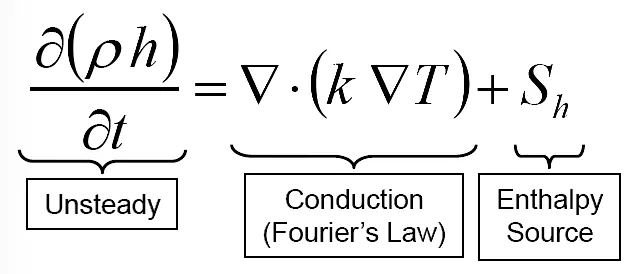
h is the enthalpy, `h=int_0^T C_p dt`

The constant of proportionality is the thermal conductivity (k). k may be a function of temperature, space, etc. For isotropic materials, k is a scalar value.

At walls, heat transfer coefficient is computed by the turbulent thermal wall functions.

HTC
The convective heat transfer coefficient is defined as, h= q_wall/(Twall - Tfluid).

Factors which affect HTC=
Temperature difference, Area, Velocity of the fluid, density, specific heat, thermal conductivity.

Heat Transfer Coefficient:

• Uses the computed wall heat flux, wall temperature, and a fluid temperature
  specified by the user
• Does not account for local variations in fluid temperature, Viscosity

Turbulence Modelling:

In a virtual wind tunnels we discretize the domain in the small elements, these elements should be small in the region where there is a gradient in the physical properties to captures its effect and get an accurate picture of flow filed. The mesh near the body is generally kept small as compared to other locations of wind tunnels since this the location where there will be more changes happening in the physical properties. The flow in the environment is always turbulent, in order to capture such a small variation in the flow we will require a large amount of mesh cells. Such a simulation is known as direct numerical simulation (DNS). But we can’t resolve such a small effect using our limited computational resources hence we need some other technique to get the turbulence effect in the flowfield.

Such an idea to get capture the turbulence was given by Sir Osborne Reynolds. In our engineering problems, we don’t need such transient and very accurate data at each time, we are more concerned with the averaged value which will definitely help us to understand some phenomena and get the numerical value of physical properties. Since the statistical quantities like mean, variance etc were reproducible, Sir Osborne Reynolds has brought up the clever idea of decomposing the randomly varying instantaneous flow property into mean plus fluctuating components. Now, substituting mean and fluctuating properties in instantaneous Navier-Stokes equations and averaging results in the so-called RANS(Reynolds averaged Navier-Stokes equations). They are the time-averaged equations of motion for fluid flow. Now there is a problem with these equations. They are not closed. There exists a "unknowns" tensor called Reynolds stress tensor. No matter how many manipulations we do,we shall always end up with more statistical unknowns than the equations relating them.This is the famous turbulence closure problem. So Reynolds Stress terms needs to be modeled using functions containing empirical constants and information about the mean flow hence known as "Turbulence Modelling".

In this simulation, we are going to use the K-omega SST turbulence model. K-omega SST (k-ω) model is one of the most commonly used models. This includes 2 additional transport equations to represent turbulent properties of flow - to account for historical effects like convection and diffusion of turbulent energy. The transport variable k determines the energy in turbulence and ω determines the scale of turbulence.
The basic k-ω model can be used for boundary layer problems, where the formulation works from the inner part through out the viscous sub-layer, till the walls - hence the k-ω SST model can be used as a low Reynolds flow application without extra damping functions. SST stands for Shear Stress Transport. The SST formulation also switches to a k-ϵ behavior in the free-stream, which avoids that the k-ω problem that the model is very sensitive to the inlet free-stream turbulence properties. The k-ω SST model also accounts for its good behaviour in adverse pressure gradients and separating flow. The k-ω SST model does produce some large turbulence levels in regions with large normal strain, like stagnation regions and regions with strong acceleration. This effect is much less pronounced than with a normal k-ϵ model though. The SST model has the ability to account for the transport of the principal shear stress in adverse pressure gradient boundary-layers.[1]

• The SST model is a hybrid two-equation model that combines the advantages of
  both k–`epsilon` and k–w models.
• k–w model performs much better than k–`epsilon` models for boundary layer flows.
  Wilcox’ original k–w model is overly sensitive to the freestream value (BC) of `omega`,
  while k–`epsilon` model is not prone to such problem.
• The k–`epsilon` and k–w models are blended such that the SST model functions like the k–ω
  close to the wall and the k–ε model in the freestream.

When using a low Reynolds turbulence model to solve the near-wall region, the first cell center must be placed in the viscous sublayer leading to the requirement of abundant mesh cells. Another way is to use the so-called wall functions, which can model the near-wall region. Wall functions are equations empirically derived and used to satisfy the physics in the near-wall region. The first cell center needs to be placed in the log-law region to ensure the accuracy of the results. Wall functions are used to bridge the inner region between the wall and the turbulence fully developed region. When using the wall functions approach, there is no need to resolve the boundary layer causing a significant reduction of the mesh size and the computational domain. As long as we are in the non-separated flow region, the results will be reasonable regardless of how the wall stress is derived. But if we decide to compute the separated flow problem, we use a low Reynolds number model or a simple algebraic model where the whole flow field is covered. This is because it can be very confusing in the separation point region where the flow direction, the sign of the wall stress, and the validity of the wall function are all unknowns. So, for separated flow problems, we move on to the low Reynolds number models like k-w SST.

Y+ is a non-dimensional distance. It is often used to describe how coarse or fine a mesh is for a particular flow pattern. It is important in turbulence modeling to determine the proper size of the cells near domain walls. The turbulence model wall laws have restrictions on the Y+ value at the wall. A non-dimensional wall distance for a wall-bounded flow can be defined in the following way

Y+ = `(Y.mu_tau)/(nu)`

`mu_tau = sqrt( tau_w/(rho))`

Where,
`mu_tau` - is the friction velocity at the nearest wall,
Y - is the distance to the nearest wall,
`nu` - is the local kinematic viscosity of the fluid.

Meshing:

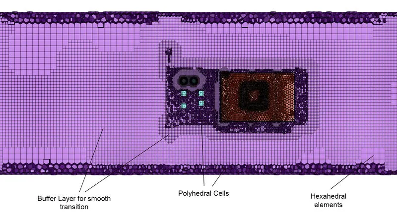
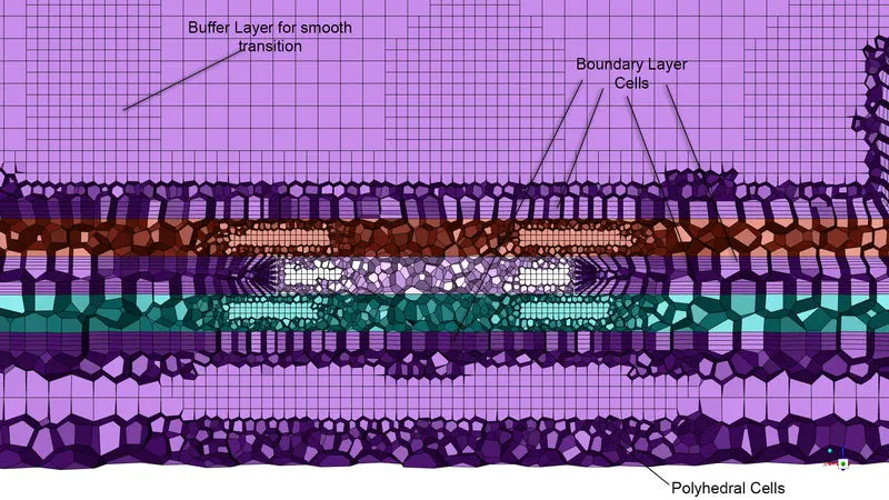
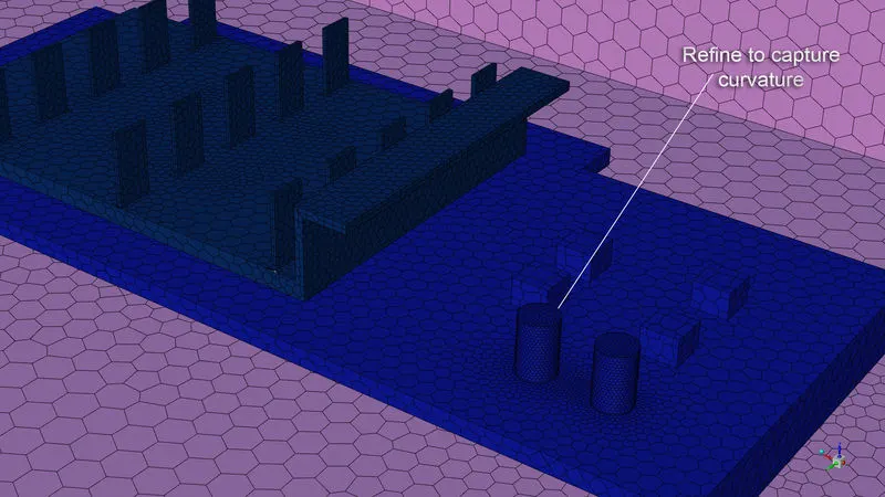
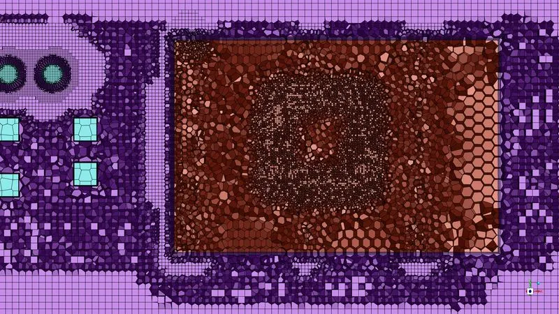
Transitioning between varying types of mesh elements in complex geometries and flow regimes has long been a major simulation challenge. Ansys Mosaic technology meets this challenge by automatically connecting different types of meshes with general polyhedral elements. Poly-Hexcore, the first application of Mosaic technology, fills the bulk region with octree hexes, keeps a high-quality layered poly-prism mesh in the boundary layer and conformally connects these two meshes with general polyhedral elements. The resulting simulation is faster with greater solution accuracy while using less RAM.

Simulation Setup:
The geometry has 1 inlet and 1 outlet. 'Velocity-inlet' boundary condition is applied at the inlet with a magnitude of 1 m/sec, 2 m/sec and 3 m/sec for the cases 1, 2, and 3 respectively. The inlet temperature of air is 298K. 'Pressure-outlet' is applied at the outlet. The operating pressure in 101325 Pa. 'Coupled-interface' is assigned at the fluid-solid interface.
The transport equations Reynolds-Averaged Navier-Stokes with `k-omega` turbulence model are solved. The first cell near the wall should be Y+ < 1. Steady-state simulation is performed until convergence is reached. SIMPLE algorithm is used for pressure-velocity coupling. The second-order scheme is used for pressure, TKE, dissipation_equation discretization.

Case 1: Velocity 1m/sec

Case 2: Velocity 3m/sec

Case 3: Velocity 5m/sec

Material Properties-

PCB
Density = 1850 kg/m3
Specific Heat Capacity, cp = 950 J/kg-k
Thermal conductivity = 0.23 W/m-k

Processor
Density = 2330 kg/m3
Specific Heat Capacity, cp = 710 J/kg-k
Thermal conductivity = 130 W/m-k

Fins
Density = 2719 kg/m3
Specific Heat Capacity, cp = 871 J/kg-k
Thermal conductivity = 202.4 W/m-k

Results:

Case 1: Velocity 1 m/s

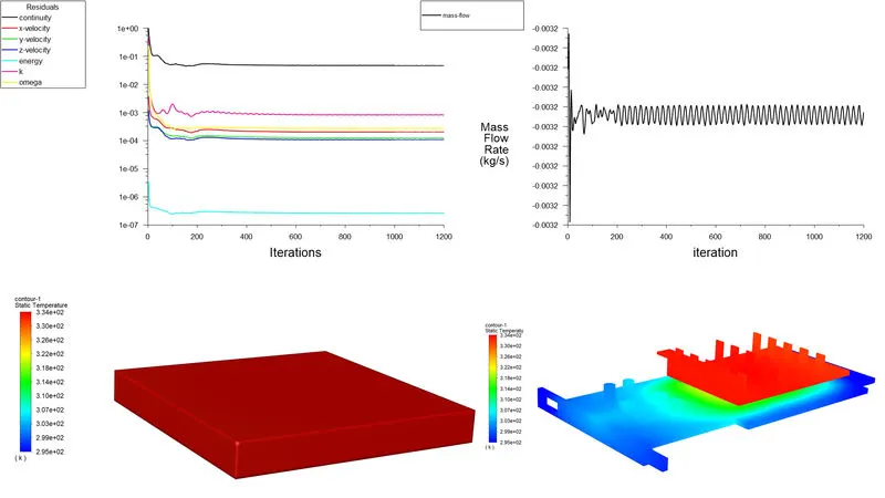
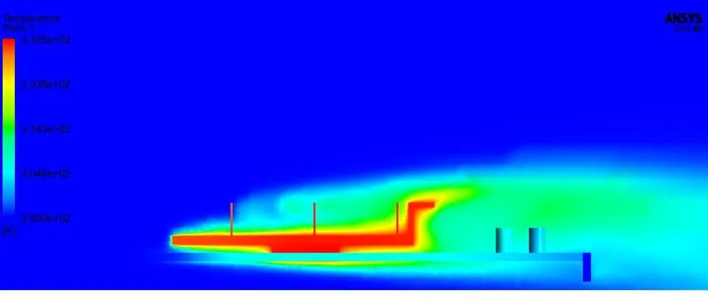
Max Temperature reached by processor= 334 K

HTC, processor = ~ 510 W/m2-K

Case 2: Velocity = 3m/s

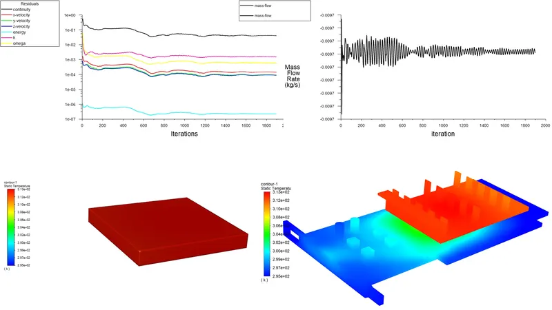
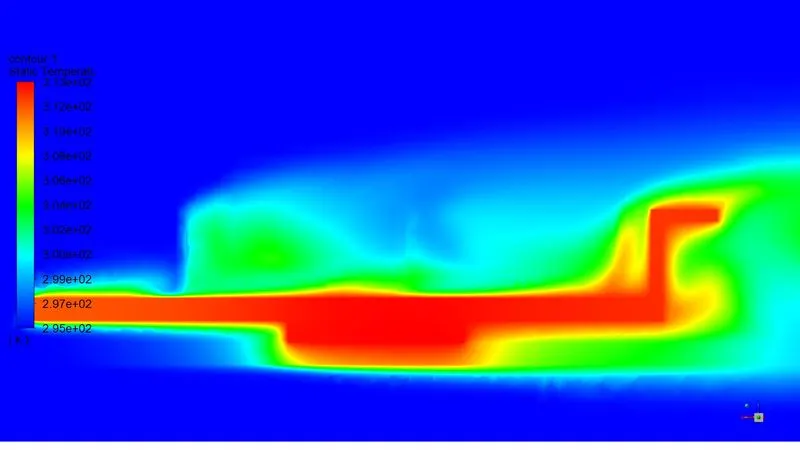
Max Temperature reached by processor = 313 K

HTC, processor = ~ 510 W/m2-K

Case 3: Velocity = 5 m/s

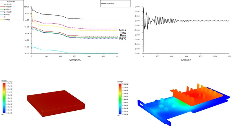
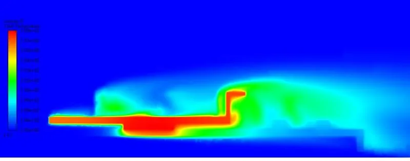
Max Temperature reached by processor= 309 K

HTC, processor = ~ 510 W/m2-K

Discussion:

• From the above contours, it is observed that the mass flow rate plot is showing oscillations, this is because the domain size is small. In order to get accurate values and convergence, we have to extend our computational domain.
• Convergence is observed by calculating Net Heat Transfer and Net Mass flow. These values should be close to zero.
• The Heat Transfer Coefficient obtained in all the cases is similar because, in Fluent, heat transfer coefficient (h) is a derived quantity using reference temperature, adjacent fluid temperature, and heat flux. In the actual scenario, the reference temperature should be the wall temperature. Therefore, the values reported by fluent will be indicative values. To get the actual h values we need to write a UDF according to our need.
• As we increase the velocity of air from 1 m/s to 5m/s the temperature of Fins decreases because the convective heat transfer increases.