Week 9 - Parametric study on Gate valve.

PARAMETRIC STUDY ON GATE VALVE

Aim:-

To Perform a parametric study on the gate valve simulation by setting the opening from 10% to 80% of the gate valve to measure the mass flow rate, flow coefficient and flow factor.

Objective:-

1. Obtain the mass flow rates at the outlet for each design point.
2. Calculate the flow coefficient and flow factor for each Opening and plot the graph.
3. Discuss the result of the mass flow rate and flow coefficient.

Introduction & Theory:-

Gate Valve:-

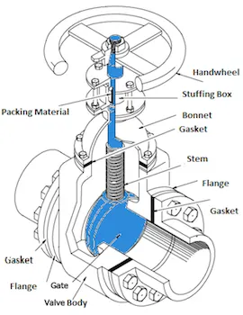
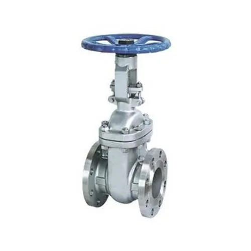
A gate valve is generally used to completely shut off fluid flow or, in the fully open position, provide full flow in a pipeline. Thus it is used either in fully closed or fully open positions. A gate valve consists of a valve body, seat and disc, a spindle, bonnet, and a wheel for operating the valve.

Parametric Study:-

• A parameter is defined as a numerical or other measurable factor forming one of a set that defines a system or set of conditions of its operation. Parameters are elements of a system that are useful for evaluating a system's performance, status, or condition. As an example parameters of an equation modelling movement could include the mechanics, masses, dimensions and shapes and densities and viscosities of fluids within the system.
• A parametric analysis, also known as a sensitivity analysis, is the study of the influence of different geometric or physical parameters or both on the solution of the problem.

Mass Flow Rate:-

Mass flow rate is the mass of a substance which passes per unit of time. Its unit is a kilogram per second [`Kg//s`].

Mass flow rate `dot m = rho.A.V`

where,

• ρ = Density of the fluid [`Kg//m^3`].
• A = Cross-sectional area of the fluid [`m^2`].
• V = Velocity of the fluid [`m//s`].

Flow Coefficient:-

The flow coefficient of a device is a relative measure of its efficiency at allowing fluid flow. It describes the relationship between the pressure drop across an orifice valve or other assembly and the corresponding flow rate

`C_v = Qsqrt((SG)/(DeltaP))`

Where,

• Q = Rate of flow (expressed in US gallons per minute)
• SG = Specific gravity of the Fluid (for water = 1)
• ΔP = The pressure drop across the valve (expressed in psi).

Flow Factor:-

The metric equivalent flow factor is calculated using metric units.

`K_v = Qsqrt((SG)/(DeltaP))`

where,

• Kv = The flow factor (expressed in [`m^3//h`])
• Q = The flow rate (expressed in [`m^3//h`])
• SG = Specific Gravity of the fluid (for water = 1)
• ΔP = The differential pressure across the device (expressed in [bar]).

Relation Between `C_v and K_V`:-

`K_v = 0.865 . C_v`

`therefore C_v = K_v/0.865`

________________________________________________________________________________

Simulation Process:-

SpaceClaim:-

• In SpaceClaim, the gate valve has been imported.
• The fluid volume is extracted by using the 'volume extracted' command.
• The Inlet and Outlet area is extruded for 800mm by using the 'Pull' command.
• The gate disk is lifted 10mm opening and set parameter in group option.
• And Select the Fluid volume and update the current body.

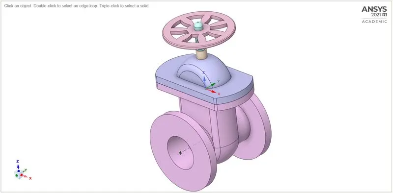
Fig(a). Gate Valve

Components:-

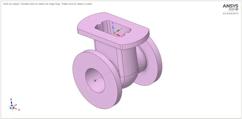
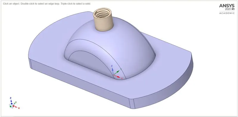
Fig(b). Bottom Fig(c). Bonnet

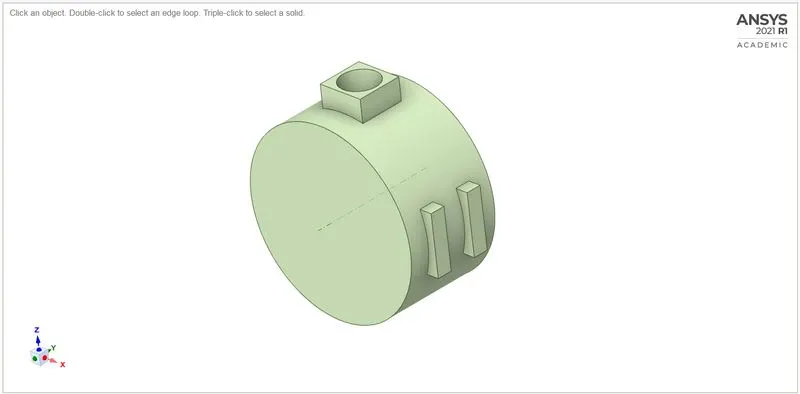
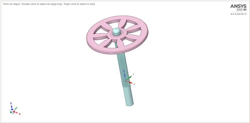
Fig(d). Gate Disk Fig(e). Spindle and Handwheel

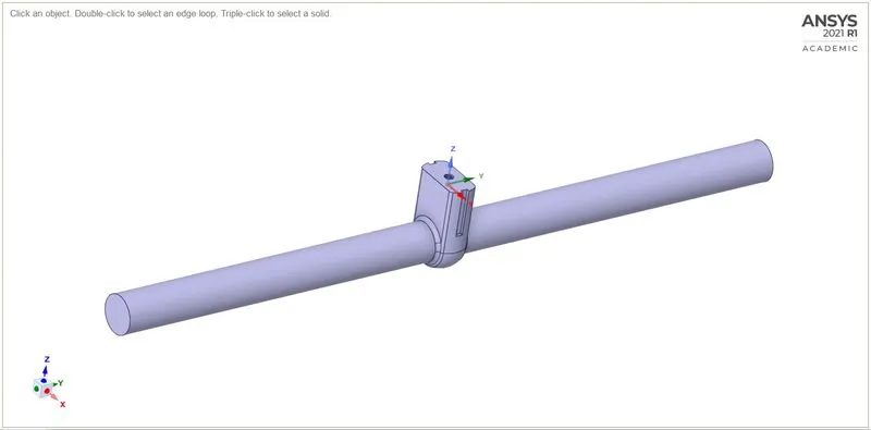
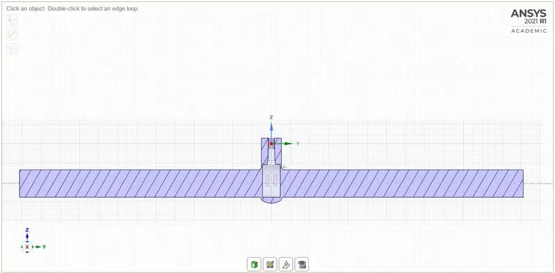
Fig(f). Fluid Volume Fig(g). Cross-Sectional View of update current body

Meshing:-

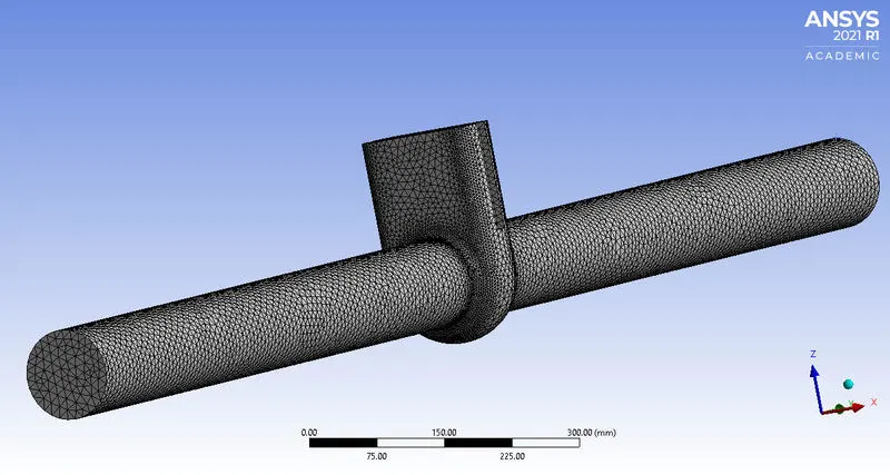
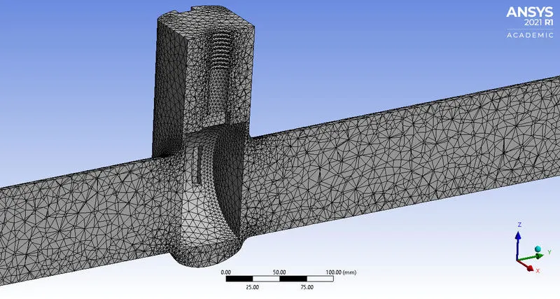
Detail of mesh:-

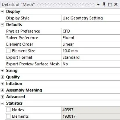
• Element Size = 10 mm
• Nodes = 40397
• No of Elements =193017

Named Selection:-

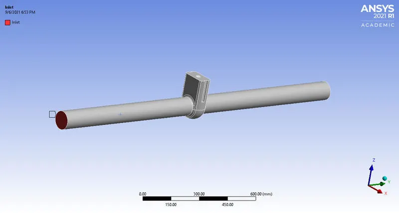
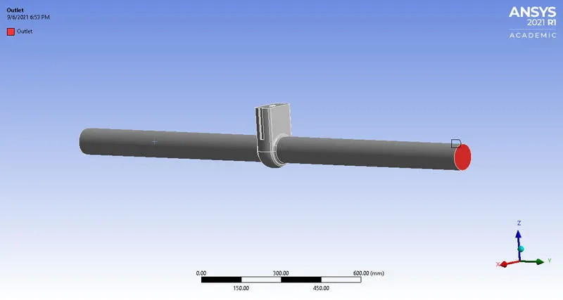
Fig(a). Inlet Fig(b). Outlet

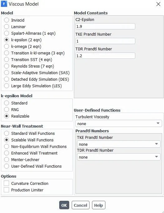
Fluent Setup:-

1. Gravity = -9.81`m//s^2` in Z-Direction

2. Viscous Model = K-epsilon, Realizable, Scalable wall function.

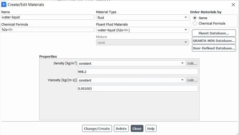
3. Material:-

The fluid material is used as water-liquid(`H_2O`)

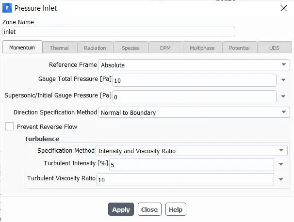
4. Boundary Condition:-

• Inlet- Pressure Inlet
• Outlet - Pressure Outlet
• Wall

5. Initialization

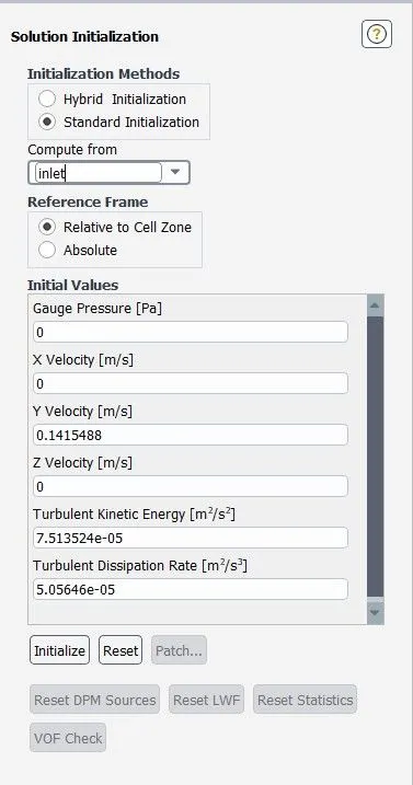
• Standard initialization is used.
• Compute from the Inlet zone.
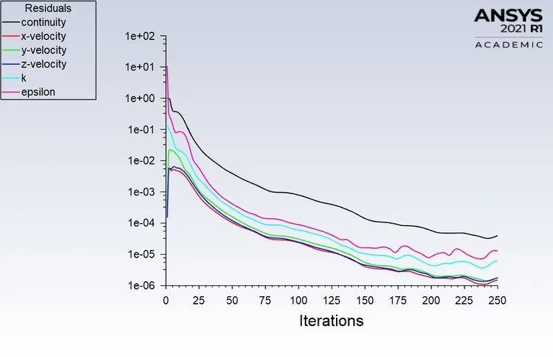
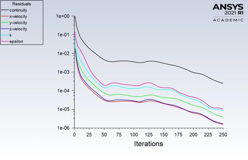
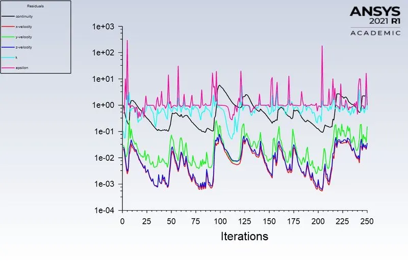
• Run for 250 iterations.

Parametric Result:-

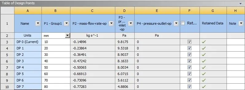
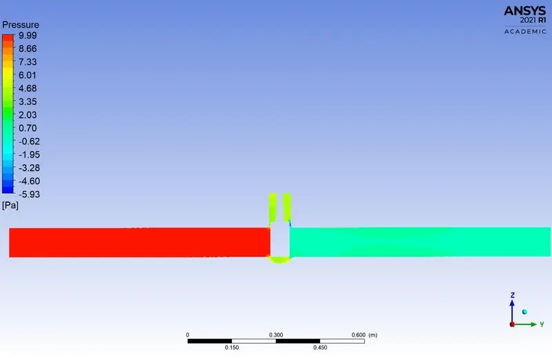
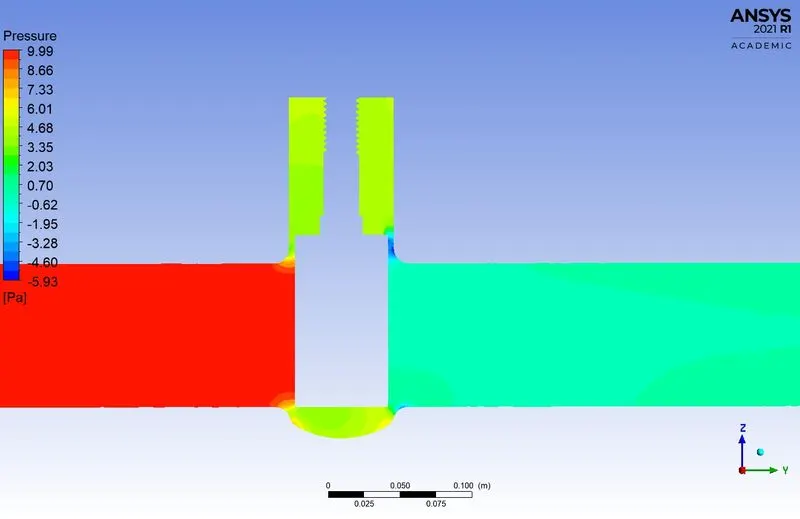
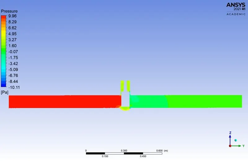
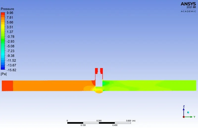
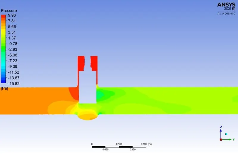
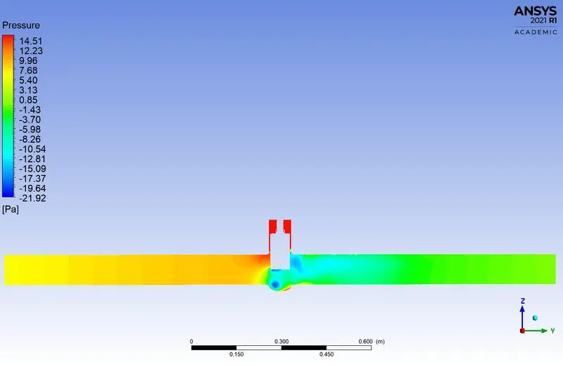
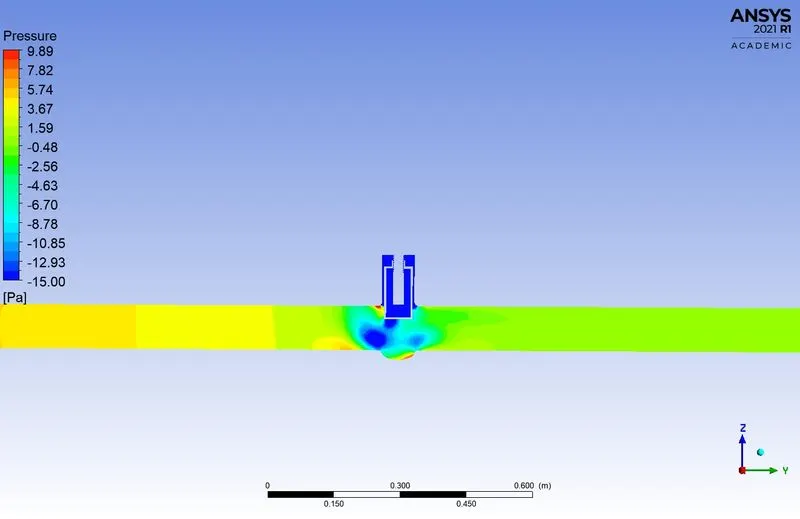
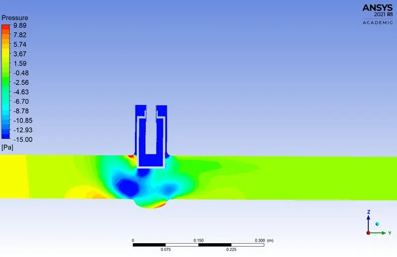
• The pressure at the inlet is 10 Pa, from the above table the inlet pressure is Static pressure.
• In a pipe flow, the static pressure and dynamic pressure is equal to 10 Pa.

Unit Conversion

• To find the flow factor the mass flow rate(Q) in expressed in [`m^3//h`].
• The Pressure Difference (ΔP) is expressed in [Bar].

Mass Flow rate (Q):-

`"1 m^3 = 1000 Kg"`

`"1 m^3/s = 1000 Kg/s"` [`"1 m^3/s = 3600 m^3/h"`]

`therefore``"1000 Kg/s = 3600 m^3/h"` [`-:``"by 1000"`]

`"1 Kg/s = 3.6 m^3/h"`

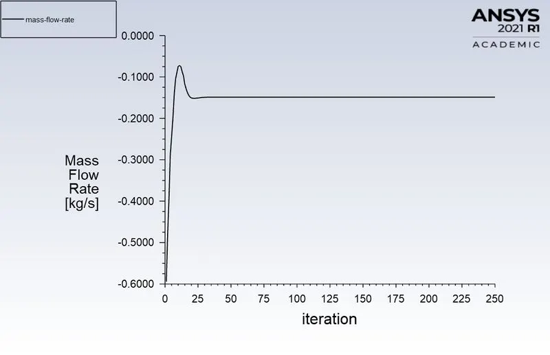
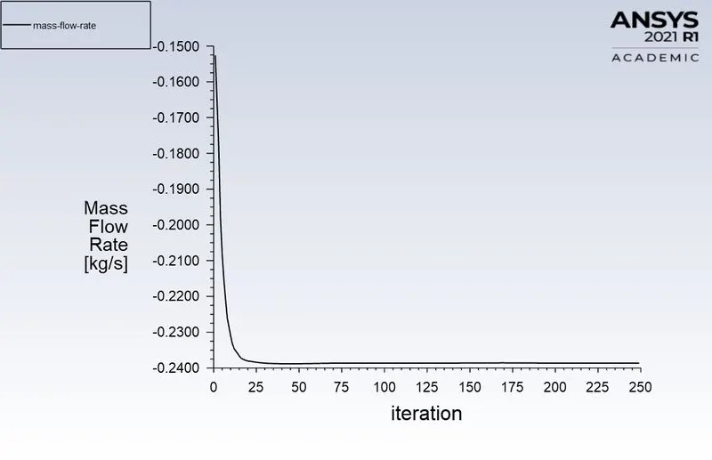
• `"0.1489 Kg/s" => 3.6 xx 0.1489 => "0.5360 m^3/h"`
• `"0.2386 Kg/s" => 3.6 xx 0.2386 => "0.8589 m^3/h"`
• `"0.3649 Kg/s" => 3.6 xx 0.3649 => "1.3136 m^3/h"`
• `"0.4724 Kg/s" => 3.6 xx 0.4724 => "1.7006 m^3/h"`
• `"0.5006 Kg/s" => 3.6 xx 0.5006 => "1.8022 m^3/h"`
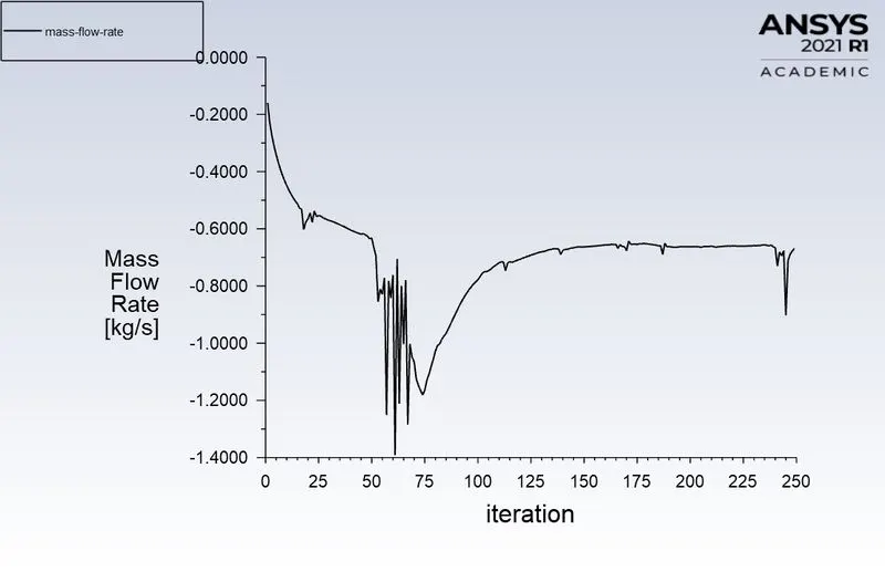
• `"0.6691 Kg/s" => 3.6 xx 0.6691 => "2.4087 m^3/h"`
• `"0.7309 Kg/s" => 3.6 xx 0.7309 => "2.6312 m^3/h"`
• `"0.7728 Kg/s" => 3.6 xx 0.7728 => "2.7820 m^3/h"`

Pressure Difference (ΔP):-

`"Pressure Diference = Inlet - Outlet"`

`"Pressure Difference = (10 - 0)"`

`therefore DeltaP = "10 Pascal"`

Here, the outlet pressure is zero. So the inlet pressure is equal to pressure difference.

`"1 Pascal = 0.00001 Bar"`

`"10 Pascal" => 0.00001 xx 10 => "0.0001 Bar"`

________________________________________________________________________________________________________________________________________________________________________

Case - 1:- 10% Opening

The Diameter of the pipe is 100 mm. So for 10% of the opening is equal to 10 mm.

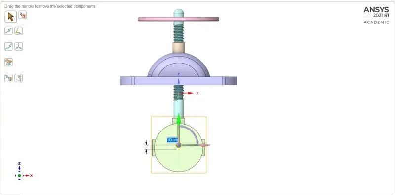
Fig(a). 10% Opening of Gate disk

Flow factor (`K_v`):-

`K_v = Qsqrt((SG)/(DeltaP))`

Here, Kv is expressed as [`m^3//h`] and ΔP as [bar].

`K_v = 0.5360 sqrt ((1)/(0.0001))`

`therefore K_v = 53.6`

Flow Coefficient (`C_v`):-

`C_v = K_v/0.865`

`C_v = 53.6/0.865`

`therefore C_v = 61.97`

Residuals:-

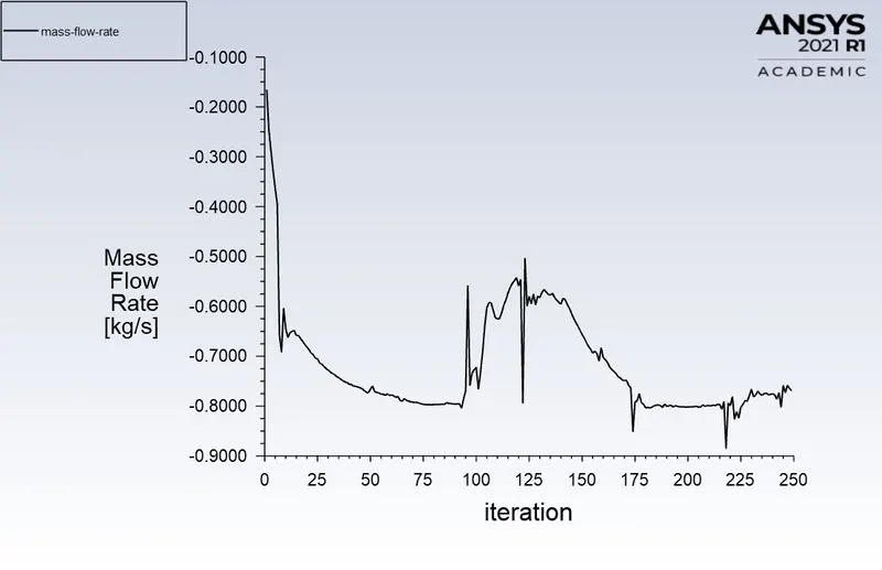
Mass Flow Rate:-

Pressure:-

________________________________________________________________________________________________________________________________________________________________________

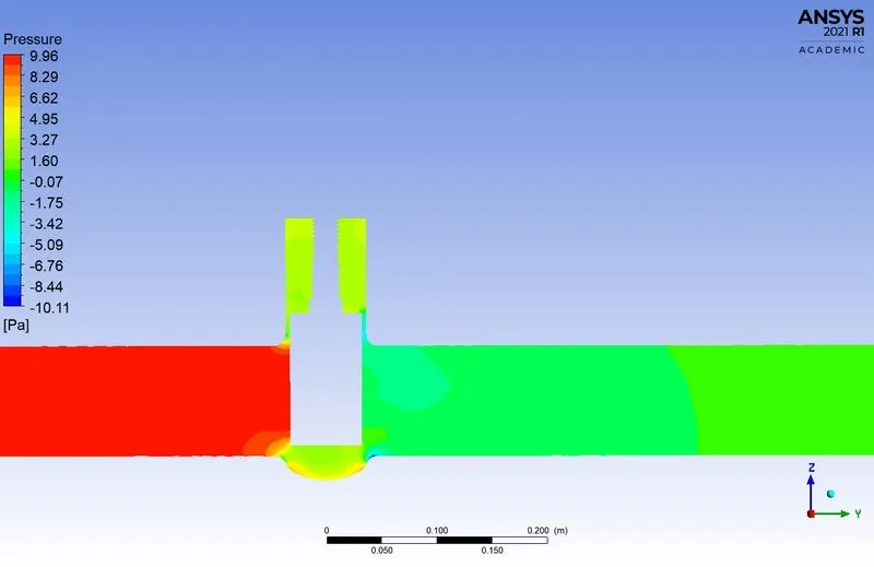
Case - 2:- 20 % Opening

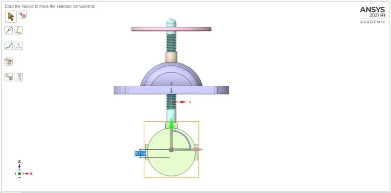
Fig(a). 20% Opening of Gate disk

Flow factor (`K_v`):-

`K_v = Qsqrt((SG)/(DeltaP))`

Here, Kv is expressed as [`m^3//h`] and ΔP as [bar].

`K_v = 0.8589 sqrt ((1)/(0.0001))`

`therefore K_v = 85.89`

Flow Coefficient (`C_v`):-

`C_v = K_v/0.865`

`C_v = 85.89/0.865`

`therefore C_v = 99.29`

Residuals:-

Mass Flow Rate:-

Pressure:-

________________________________________________________________________________________________________________________________________________________________________

Case - 3:- 30 % Opening

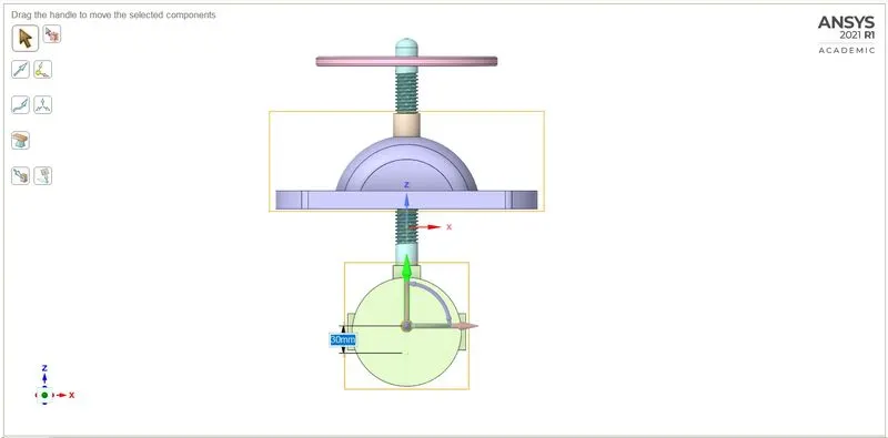
Fig(a). 30% Opening of Gate disk

Flow factor (`K_v`):-

`K_v = Qsqrt((SG)/(DeltaP))`

Here, Kv is expressed as [`m^3//h`] and ΔP as [bar].

`K_v = 1.3136 sqrt ((1)/(0.0001))`

`therefore K_v = 131.36`

Flow Coefficient (`C_v`):-

`C_v = K_v/0.865`

`C_v = 131.36/0.865`

`therefore C_v = 151.86`

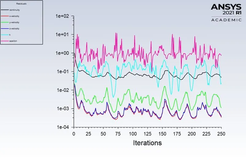
Residuals:-

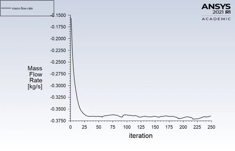
Mass Flow Rate:-

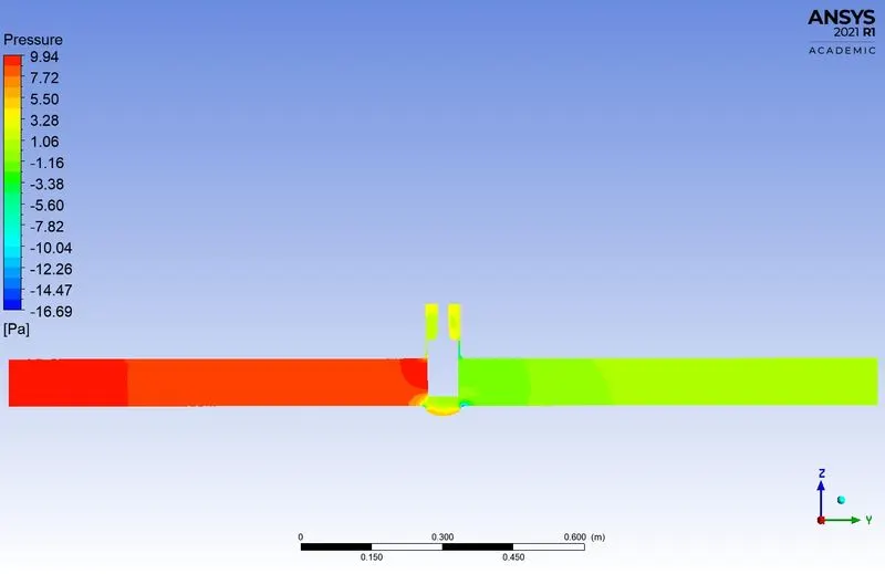
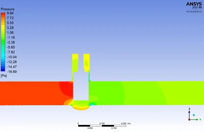
Pressure:-

________________________________________________________________________________________________________________________________________________________________________

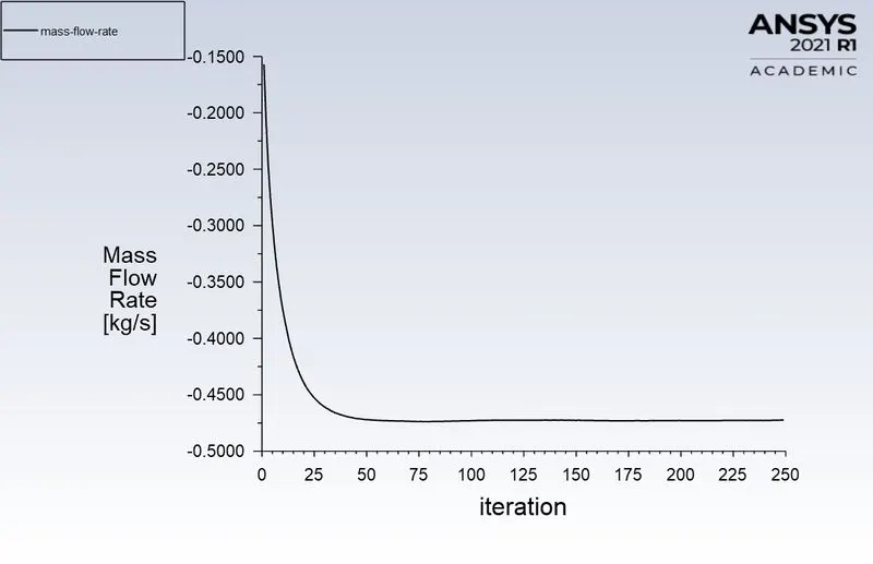
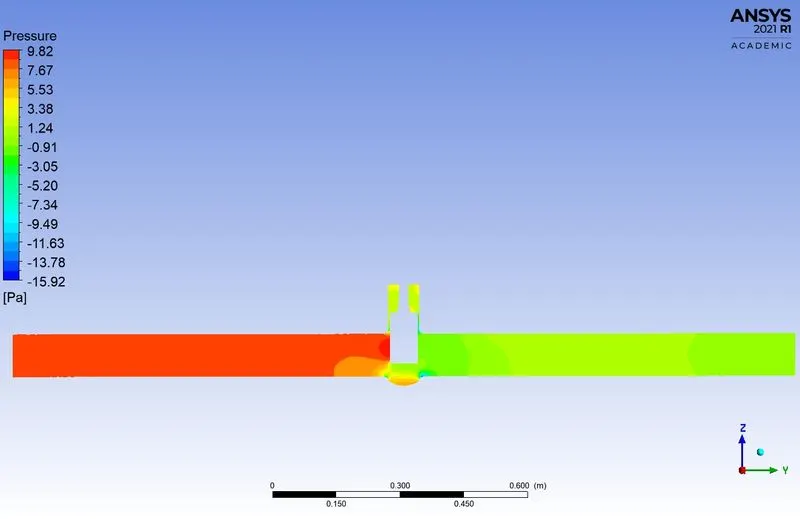
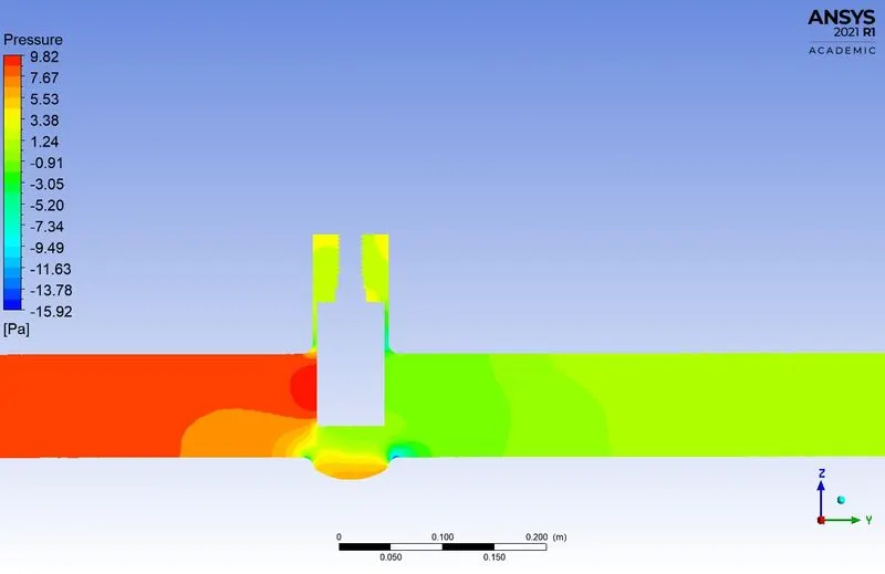
Case - 4:- 40 % Opening

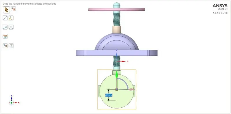
Fig(a). 40% Opening of Gate disk

Flow factor (`K_v`):-

`K_v = Qsqrt((SG)/(DeltaP))`

Here, Kv is expressed as [`m^3//h`] and ΔP as [bar].

`K_v = 1.7006 sqrt ((1)/(0.0001))`

`therefore K_v = 170.06`

Flow Coefficient (`C_v`):-

`C_v = K_v/0.865`

`C_v = 170.06/0.865`

`therefore C_v = 196.60`

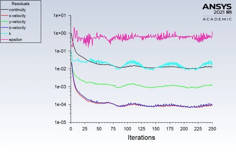
Residuals:-

Mass Flow Rate:-

Pressure:-

________________________________________________________________________________________________________________________________________________________________________

Case - 5:- 50 % Opening

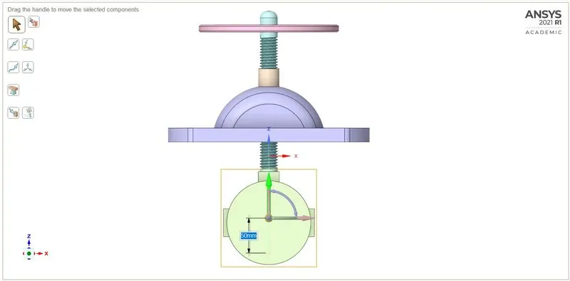
Fig(a). 50% Opening of Gate disk

Flow factor (`K_v`):-

`K_v = Qsqrt((SG)/(DeltaP))`

Here, Kv is expressed as [`m^3//h`] and ΔP as [bar].

`K_v = 1.8022 sqrt ((1)/(0.0001))`

`therefore K_v = 180.22`

Flow Coefficient (`C_v`):-

`C_v = K_v/0.865`

`C_v = 180.22/0.865`

`therefore C_v = 208.34`

Residuals:-

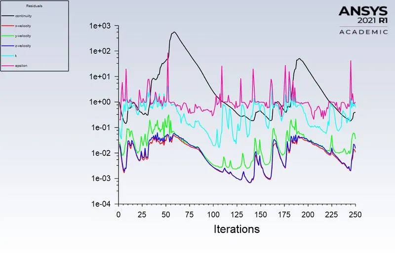
Mass Flow Rate:-

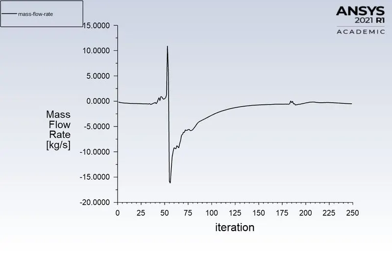
Pressure:-

________________________________________________________________________________________________________________________________________________________________________

Case - 6:- 60 % Opening

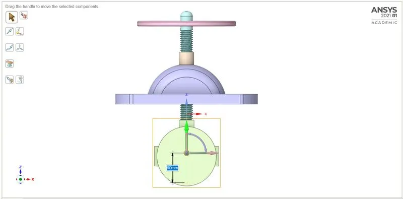
Fig(a). 60% Opening of Gate disk

Flow factor (`K_v`):-

`K_v = Qsqrt((SG)/(DeltaP))`

Here, Kv is expressed as [`m^3//h`] and ΔP as [bar].

`K_v = 2.4087 sqrt ((1)/(0.0001))`

`therefore K_v = 240.87`

Flow Coefficient (`C_v`):-

`C_v = K_v/0.865`

`C_v = 240.87/0.865`

`therefore C_v = 278.46`

Residuals:-

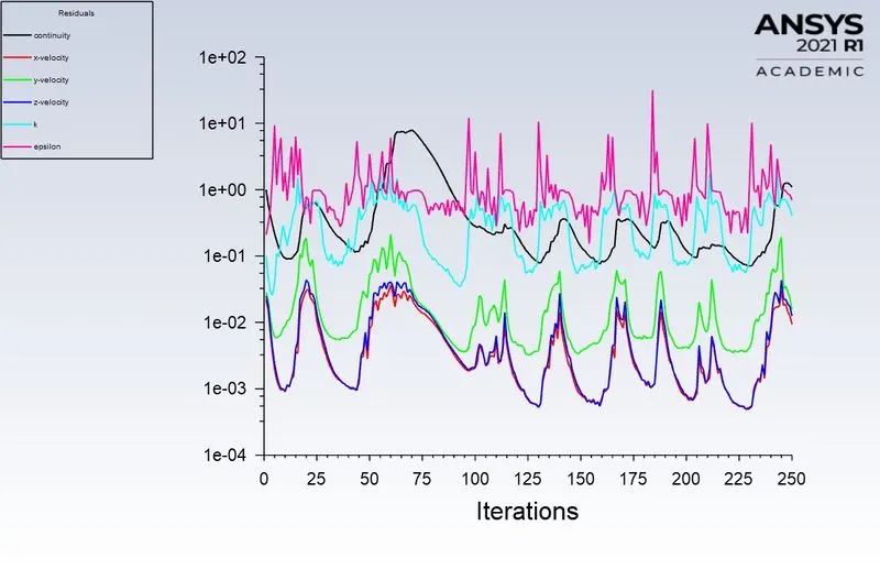
Mass Flow Rate:-

Pressure:-

________________________________________________________________________________________________________________________________________________________________________

Case - 7:- 70 % Opening

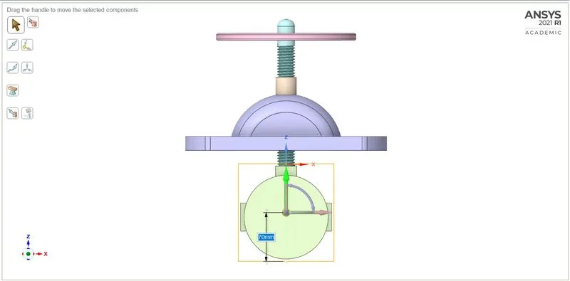
Fig(a). 70% Opening of Gate disk

Flow factor (`K_v`):-

`K_v = Qsqrt((SG)/(DeltaP))`

Here, Kv is expressed as [`m^3//h`] and ΔP as [bar].

`K_v = 2.6312 sqrt ((1)/(0.0001))`

`therefore K_v = 263.12`

Flow Coefficient (`C_v`):-

`C_v = K_v/0.865`

`C_v = 263.12/0.865`

`therefore C_v = 304.18`

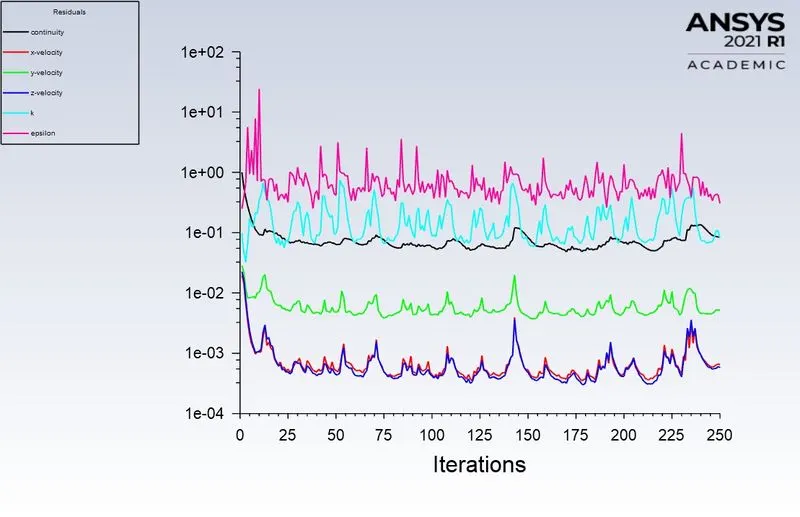
Residuals:-

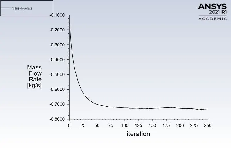
Mass Flow Rate:-

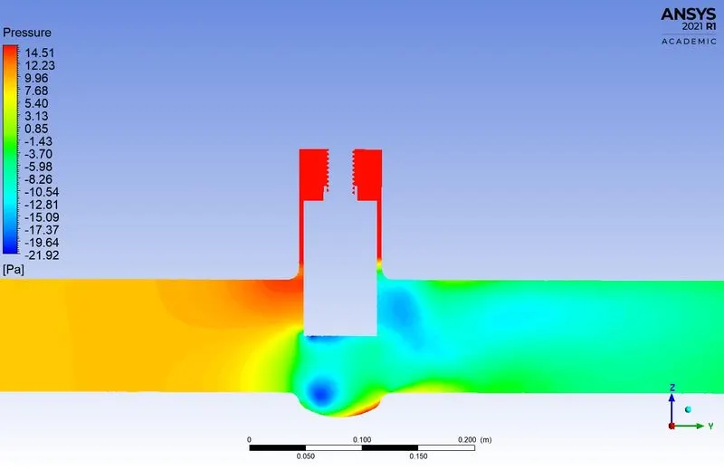
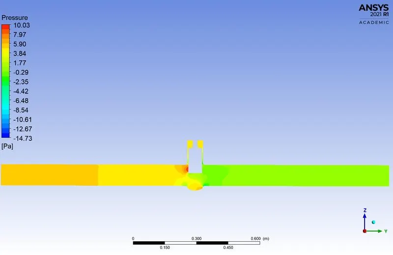
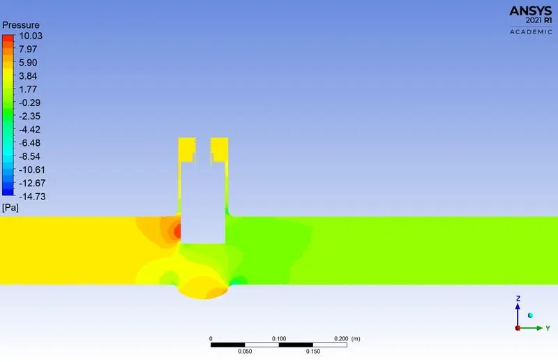
Pressure:-

________________________________________________________________________________________________________________________________________________________________________

Case - 8:- 80 % Opening

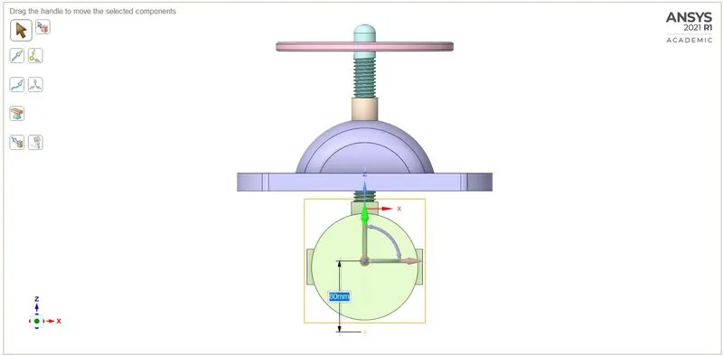
Fig(a). 10% Opening of Gate disk

Flow factor (`K_v`):-

`K_v = Qsqrt((SG)/(DeltaP))`

Here, Kv is expressed as [`m^3//h`] and ΔP as [bar].

`K_v =2.7820 sqrt ((1)/(0.0001))`

`therefore K_v = 278.2`

Flow Coefficient (`C_v`):-

`C_v = K_v/0.865`

`C_v = 278.2/0.865`

`therefore C_v = 321.61`

Residuals:-

Mass Flow Rate:-

Pressure:-

Result & Comparison:-

Tabulation:-

Valve Opening	Mass Flow Rate (`Kg//s`)	Mass Flow Rate (`m^3//hr`)	Flow Factor (`K_v`)	Flow Coefficient (`C_v`)
10 mm	0.14896	0.5360	53.6	61.97
20 mm	0.23864	0.8589	85.89	99.29
30 mm	0.36491	1.3136	131.36	151.86
40 mm	0.47242	1.7006	170.06	196.60
50 mm	0.50065	1.8002	180.22	208.34
60 mm	0.66913	2.4087	240.87	278.46
70 mm	0.73096	2.6312	263.12	304.18
80 mm	0.77283	2.7820	278.2	321.61

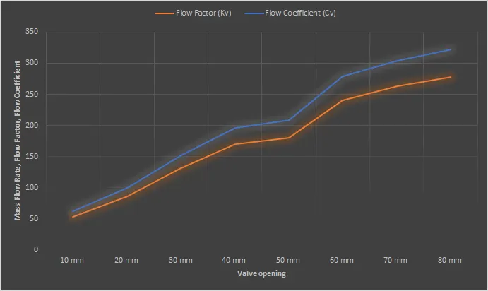
Plotted Graph for Flow Factor and Flow Coefficient:-

Conclusion:-

• From the above result and tabulation, the Mass flow rate is increased gradually when the gate valve is opening.
• The Flow factor and Flow Coefficient is calculate from the mass flow rate and pressure drop of the gate valve.
• The flow factor is in SI units and the zFlow coefficient is in US standards.
• The 10 mm opening of gate disk is simulated and prameterized the other simulation from 20 mm to 80 mm.
• To get the required data of design points to set as current. The all parameters are changed to that design points
• This parametic study is used to reduced the simulation time and operating time.
• To conclude that if we want to control the mass flow rate at outlet or orifice we can change the valve opening to get the desired mass flow rate.