Week 7 - Simulation of a 1D Super-sonic nozzle flow simulation using Macormack Method
Simulation of 1D Super-sonic Nozzle flow simulation using MaCormack Method
To simulate the Isentropic flow through a quasi 1D subsonic-supersonic nozzle for both conservation and Non-conservation forms.
- Steady-state distribution of primitive variables inside the nozzle
- Time-wise variation of the primitive variables
- Variation of Mass flow rate distribution inside the nozzle at different time steps during the time-marching process
- Comparison of Normalized mass flow rate distributions of both forms
- Perform a Grid dependence test.
Non Conservation form:-
- Continuity Equation
`(∂rho)/(∂t) = -rho(∂V)/(∂x)- rho*V(∂(ln A))/(∂x) -V(∂rho)/(∂x)`
- Momentum Equation
`(∂V)/(∂t) = -V(∂V)/(∂x)- (1/gamma)((∂T)/(∂x)+(T)/(rho)(∂rho)/(∂x))`
- Energy Equation
`(∂T)/(∂t) = -V(∂T)/(∂x) -(gamma-1)T[(∂V)/(∂x)+V(∂(ln A))/(∂x)]`
Boundary Conditions:-
- Subsonic Inflow
`V_1 = 2V_2 -V_3`
- Supersonic Outflow
`V_n = 2V_(n-1) - V_(n-2)`
`rho_n = 2rho_(n-1) - rho_(n-2)`
`T_n = 2T_(n-1) - T_(n-2)`
Nozzle Shape and Initial Condition:-
Area `A = 1 + 2.2(x-1.5)^2`
Initial Condition
Density `rho = 1 - 0.3146x`
Temperature `T = 1 - 0.2314x`
Velocity`V = (0.1 + 1.09x)T^(1/2)`
initial condition at t = 0
For ΔT = 0.0201
Function code for Non_conservation form
function [rho, t, v, nt, dt, k, mass_flow, pressure, Mach, rho_th, v_th, t_th, pressure_th, Mach_th, M_exact, p_exact, rho_exact, t_exact] = non_conservative_form(n,x,dx,gamma,throat,a)

% Calculate Initial Profiles
rho = 1 - 0.3146*x;
t = 1 - 0.2314*x;
v = (0.1 + 1.09*x).*t.^0.5;

% Time Step
nt = 1400;
dt = 0.0201;

% outer time loop

for k=1:nt
    rho_old = rho;
    v_old = v;
    t_old = t;

    % Predictor method
    for j = 2:n-1
        drho_dx = (rho(j+1) - rho(j))/dx;
        dv_dx = (v(j+1) - v(j))/dx;
        dt_dx = (t(j+1) - t(j))/dx;
        dlog_a_dx = (log(a(j+1)) - log(a(j)))/dx;

        % Continuity Equation
        drhodt_p(j) = -rho(j)*dv_dx - rho(j)*v(j)*dlog_a_dx -v(j)*drho_dx;

        % Momentum Equation
        dvdt_p(j) = -v(j)*dv_dx - (1/gamma)* (dt_dx + (t(j)/rho(j))*drho_dx);

        % Energy Equation
        dtdt_p(j) = -v(j)*dt_dx - (gamma-1)*t(j)*(dv_dx + v(j)*dlog_a_dx);

        % Solution Update
        rho(j) = rho(j) + drhodt_p(j)*dt;
        v(j) = v(j) + dvdt_p(j)*dt;
        t(j) = t(j) + dtdt_p(j)*dt;
    end

    % Corrector Method
    for j = 2:n-1
        drho_dx = (rho(j)-rho(j-1))/dx;
        dv_dx = (v(j)-v(j-1))/dx;
        dt_dx = (t(j)-t(j-1))/dx;
        dlog_a_dx = (log(a(j))-log(a(j-1)))/dx;

        % Continuity Equation
        drhodt_c(j) = -rho(j)*dv_dx-rho(j)*v(j)*dlog_a_dx -v(j)*drho_dx;

        % Momentum Equation
        dvdt_c(j) = -v(j)*dv_dx - (1/gamma)*(dt_dx + (t(j)/rho(j))*drho_dx);

        % Energy equation
        dtdt_c(j) = -v(j)*dt_dx - (gamma-1)*t(j)*(dv_dx + v(j)*dlog_a_dx);
    end

    % Compute the average time derivative
    drhodt = 0.5*(drhodt_p + drhodt_c);
    dvdt = 0.5*(dvdt_p + dvdt_c);
    dtdt = 0.5*(dtdt_p + dtdt_c);

    % Final solution update
    for i = 2:n-1
        rho(i) = rho_old(i) + drhodt(i)*dt;
        v(i) = v_old(i) + dvdt(i)*dt;
        t(i) = t_old(i) + dtdt(i)*dt;
    end

    % Applying Boundary Condition
    % Inlet
    v(1) = 2*v(2) - v(3);

    % Outlet
    rho(n) = 2*rho(n-1) - rho(n-2);
    v(n) = 2*v(n-1) - v(n-2);
    t(n) = 2*t(n-1) - t(n-2);

    % Mass Flow rate
    mass_flow = rho.*a.*v;

    % Pressure Ratio
    pressure = rho.*t;

    % Mach number
    Mach = v./sqrt(t);

    % At throat section
    rho_th(k) = rho(throat);
    v_th(k) = v(throat);
    t_th(k) = t(throat);
    pressure_th(k) = pressure(throat);
    Mach_th(k) = Mach(throat);

    % Exact Solution
    M_exact = 1*ones(1,1400);
    p_exact = 0.528*ones(1,1400);
    rho_exact = 0.634*ones(1,1400);
    t_exact = 0.833*ones(1,1400);

    % Non Dimentional Mass Flow Rate
    figure(1)
    hold on
    if k == 1
        plot(x,mass_flow,'r','linewidth',2)
    elseif k == 50
        plot(x,mass_flow,'g','linewidth',2)
    elseif k == 100
        plot(x,mass_flow,'y','linewidth',2)
    elseif k == 150
        plot(x,mass_flow,'c','linewidth',2)
    elseif k == 200
        plot(x,mass_flow,'k','linewidth',2)
    elseif k == 700
        plot(x,mass_flow,'--','linewidth',2)

    xlabel('Non-dimensional Distance Through Nozzle(x)')
    ylabel('Non-dimensional Mass Flow')
    legend('1dt','50dt','100dt','150dt','200dt','700dt')
    title('Variation of Mass flow rate at different time step during time-marching at Non-conservation form','Fontweight','bold')
    grid on
    end

end

    % Qualitative aspects of the 1D nozzle flow

    figure(2)
    subplot(4,1,1)
    plot(x,Mach,'m','linewidth',2)
    ylabel('Mach Number')
    legend('Mach Number','location','best')
    title('Qualitative aspects of Quasi-One-Dimensional Nozzle Flow for Non-conservation form','Fontweight','bold')

    subplot(4,1,2)
    plot(x,pressure,'y','linewidth',2)
    ylabel('{p/p0}')
    legend('Pressure Ratio','location','best')

    subplot(4,1,3)
    plot(x,rho,'g','linewidth',2)
    ylabel('{rho/rho0}')
    legend('Density Ratio','location','best')

    subplot(4,1,4)
    plot(x,t,'c','linewidth',2)
    xlabel('Non-dimensional Distance Through Nozzle(x)')
    ylabel('{T/T0}')
    legend('Temperature Ratio','location','best')

    % Timewise variation of primitive variables at the throat
    figure(3)

    subplot(4,1,1)
    grid on
    plot(rho_th,'linewidth',2)
    hold on
    plot(rho_exact,'linewidth',2)
    ylabel('Density')
    legend('Numerical Result','Exact result')
    title('Density Variation at Throat')

    subplot(4,1,2)
    grid on
    plot(t_th,'linewidth',2)
    hold on
    plot(t_exact,'linewidth',2)
    ylabel('Temperature')
    legend('Numerical Result','Exact result')
    title('Temperature Variation at Throat')

    subplot(4,1,3)
    grid on
    plot(pressure_th,'linewidth',2)
    hold on
    plot(p_exact,'linewidth',2)
    ylabel('Pressure')
    legend('Numerical Result','Exact result')
    title('Pressure Variation at Throat')

    subplot(4,1,4)
    grid on
    plot(Mach_th,'linewidth',2)
    hold on
    plot(M_exact,'linewidth',2)
    xlabel('Number of Time Step')
    ylabel('Mach Number')
    legend('Numerical Result','Exact result')
    title('Mach Number Variation at Throat')
end
Plotted graph for Non-Conservation Form:-
1. Variation of Mass Flow rate distribution inside the nozzle at different time steps during the time-marching process.
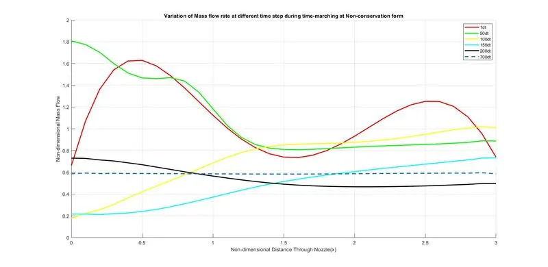
The above graph represents the mass flow at different time steps. However, the mass flow rate reaches the steady-state at the 700th time step.
2. Steady-state distribution of primitive variables inside the nozzle
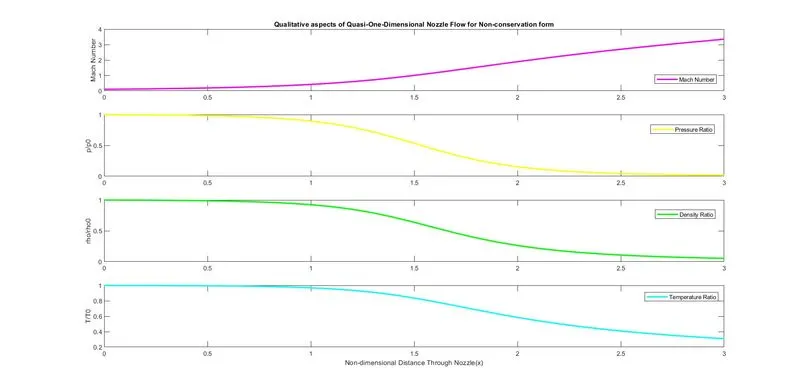
The above quasi-one-dimensional nozzle flow of Non-Conservative form shows that the primitive variables like Density, Temperature, Pressure, and Mach number from subsonic to supersonic through nozzle distance.
3. Time-wise variation of primitive variables
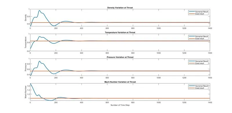
The above graph is a comparison of the Numerical results and Exact results of The Time-wise variation of the Density, Temperature, Pressure, and Mach number at the nozzle throat through the different time steps.
Conservation form:-
- Continuity Equation
`(∂rhoA)/(∂t) = -(∂(rhoAV))/(∂x)`
- Momentum Equation
`(∂(rhoAV))/(∂t) = -(∂[rhoAV +(1/gamma)pa)]/(∂x) + (1/gamma)p(∂A)/(∂x)`
- Energy Equation
`(∂[rho(e/(gamma-1) + gamma/2 V^2)A])/(∂t) = -(∂[rho(e/(gamma-1) + gamma/2 V^2) VA +rhoAV])/(∂x)`
Boundary Conditions:-
- Inflow Boundary
`U_1 = A(1)`
`U_2 = 2U_2(2) -U_2(3)`
`U_3 = U1(T/(gamma-1) +gamma/2 V^2)`
- Outflow Boundary
`U_1(n) = 2U_1(n-1) - U_1(n-2)`
`U_2(n) = 2U_2(n-1) - U_2(n-2)`
`U_3(n) = 2U_3(n-1) - U_3(n-2)`
Initial Conditions:-
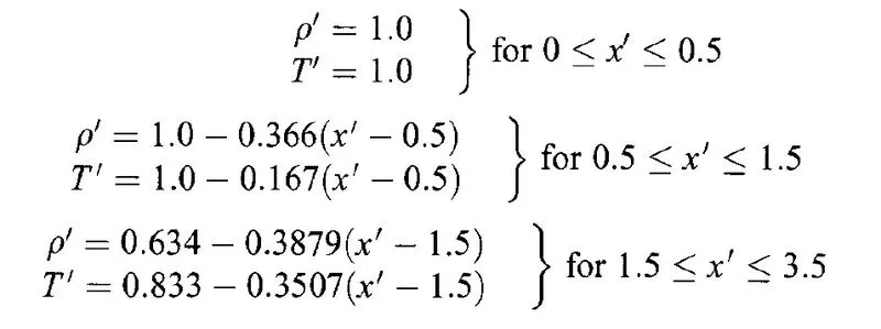
`U_1 = rho*A`
`U_2 = rho*A*V`
`U_3 = rho(e/(gamma-1) +gamma/2 V^2) A`
`V = (0.59)/(rhoA)`
For ΔT = 0.0267
Function code for Conservation Form
function[nt_c, dt_c, l, rho_c, t_c, v_c, mass_flow_c, pressure_c, Mach_c, rho_c_th, v_c_th, t_c_th, pressure_c_th, Mach_c_th, M_exact, p_exact, rho_exact, t_exact] = conservative_form(n,x,dx,gamma,throat,a)

% Time Step
nt_c = 1400;
dt_c = 0.0267;

% Initial Condition for Conservative form
for z = 1:n
    if(x(z)>=0 && x(z)<=0.5)
        rho_c(z) = 1;
        t_c(z)= 1;
    elseif(x(z)>=0.5 && x(z)<=1.5)
        rho_c(z) = 1-0.366*(x(z)-0.5);
        t_c(z) = 1-0.167*(x(z)-0.5);
    elseif(x(z)>=1.5 && x(z)<=3.5)
        rho_c(z) = 0.634-0.3879*(x(z)-1.5);
        t_c(z) = 0.833-0.3507*(x(z)-1.5);
    end
end

% Solution Vector

v_c = 0.59./(rho_c.*a);
U1 = rho_c.*a;
U2 = rho_c.*a.*v_c;
U3 = rho_c.*((t_c/(gamma-1))+(gamma/2).*(v_c.^2)).*a;

% outer time loop

for l = 1:nt_c
    U1_old = U1;
    U2_old = U2;
    U3_old = U3;

    % Flux Vector
    F1 = U2;
    F2 = (U2.^2./U1)+((gamma-1)/(gamma)*(U3-(gamma*U2.^2)./(2*U1)));
    F3 = ((gamma*(U2.*U3)./U1))-((gamma*(gamma-1))/2)*((U2.^3)./(U1.^2));

    % Predictor Method
    for j = 2:n-1
        J2_p(j) = (1/gamma)*(rho_c(j)*t_c(j))*((a(j+1)-a(j))/dx);
        % using forward differences
        dU1dt_p(j) = -(F1(j+1)-F1(j))/dx;
        dU2dt_p(j) = (-(F2(j+1)-F2(j))/dx)+J2_p(j);
        dU3dt_p(j) = -(F3(j+1)-F3(j))/dx;


        % Solution Update
        U1(j) = U1(j) + dU1dt_p(j)*dt_c;
        U2(j) = U2(j) + dU2dt_p(j)*dt_c;
        U3(j) = U3(j) + dU3dt_p(j)*dt_c;
    end

    % Updating values
    rho_c = (U1./a);
    v_c = (U2./U1);
    t_c = (gamma-1)*((U3./U1)-(gamma/2)*(v_c.^2));

    % Flux Vector
    F1 = U2;
    F2 = (U2.^2./U1)+((gamma-1)/(gamma)*(U3-(gamma*U2.^2)./(2*U1)));
    F3 = ((gamma*(U2.*U3)./U1))-((gamma*(gamma-1))/2)*((U2.^3)./(U1.^2));

    % Corrector Method
    for j = 2:n-1
        J2_c(j) = (1/gamma)*(rho_c(j)*t_c(j))*((a(j)-a(j-1))/dx);
        % using backward differences
        dU1dt_c(j) = -(F1(j)-F1(j-1))/dx;
        dU2dt_c(j) = (-(F2(j)-F2(j-1))/dx)+J2_c(j);
        dU3dt_c(j) = -(F3(j)-F3(j-1))/dx;
    end

    % Compute the average time derivative
    dU1dt_avg = 0.5*(dU1dt_p + dU1dt_c);
    dU2dt_avg = 0.5*(dU2dt_p + dU2dt_c);
    dU3dt_avg = 0.5*(dU3dt_p + dU3dt_c);

    % Final solution update
    for i = 2:n-1
        U1(i) = U1_old(i) + dU1dt_avg(i)*dt_c;
        U2(i) = U2_old(i) + dU2dt_avg(i)*dt_c;
        U3(i) = U3_old(i) + dU3dt_avg(i)*dt_c;
    end

    % Applying Boundary Condition
    % Inlet
    U1(1) = a(1);
    U2(1) = 2*U2(2) - U2(3);
    U3(1) = U1(1)*((t_c(1)/(gamma-1)) + (gamma/2)*(v_c(1)^2));

    % Outlet
    U1(n) = 2*U1(n-1) - U1(n-2);
    U2(n) = 2*U2(n-1) - U2(n-2);
    U3(n) = 2*U3(n-1) - U3(n-2);

    % Updating values
    rho_c = (U1./a);
    v_c = (U2./U1);
    t_c = (gamma-1)*((U3./U1)-(gamma/2)*(v_c.^2));

    % Mass Flow rate
    mass_flow_c = rho_c.*a.*v_c;

    % Pressure Ratio
    pressure_c = rho_c.*t_c;

    % Mach number
    Mach_c = v_c./sqrt(t_c);

    % At throat section
    rho_c_th(l) = rho_c(throat);
    v_c_th(l) = v_c(throat);
    t_c_th(l) = t_c(throat);
    pressure_c_th(l) = pressure_c(throat);
    Mach_c_th(l) = Mach_c(throat);

    % Exact Solution
    M_exact = 1*ones(1,1400);
    p_exact = 0.528*ones(1,1400);
    rho_exact = 0.634*ones(1,1400);
    t_exact = 0.833*ones(1,1400);

    % Non Dimentional Mass Flow Rate
    figure(4)
    hold on
    if l == 1
        plot(x,mass_flow_c,'r','linewidth',2)
    elseif l == 100
        plot(x,mass_flow_c,'g','linewidth',2)
    elseif l == 200
        plot(x,mass_flow_c,'c','linewidth',2)
    elseif l == 700
        plot(x,mass_flow_c,'k','linewidth',2)

    xlabel('Non-dimensional Distance Through Nozzle(x)')
    ylabel('Non-dimensional Mass Flow')
    legend('1dt','100dt','200dt','700dt')
    title('Variation of Mass flow rate at different time step during time-marching at Conservation form','Fontweight','bold')
    grid on
    end

end

   % Qualitative aspects of the 1D nozzle flow
    figure(5)
    subplot(4,1,1)
    plot(x,Mach_c,'m','linewidth',2)
    ylabel('Mach Number')
    legend('Mach Number','location','best')
    title('Qualitative aspects of Quasi-One-Dimensional Nozzle Flow for Conservation form','Fontweight','bold')

    subplot(4,1,2)
    plot(x,pressure_c,'y','linewidth',2)
    ylabel('{p/p0}')
    legend('Pressure Ratio','location','best')

    subplot(4,1,3)
    plot(x,rho_c,'g','linewidth',2)
    ylabel('{rho/rho0}')
    legend('Density Ratio','location','best')

    subplot(4,1,4)
    plot(x,t_c,'c','linewidth',2)
    xlabel('Non-dimensional Distance Through Nozzle(x)')
    ylabel('{T/T0}')
    legend('Temperature Ratio','location','best')

     % Timewise variation of primitive variables at the throat
    figure(6)

    subplot(4,1,1)
    grid on
    plot(rho_c_th,'linewidth',2)
    hold on
    plot(rho_exact,'linewidth',2)
    ylabel('Density')
    legend('Numerical Result','Exact result')
    title('Density Variation at Throat')

    subplot(4,1,2)
    grid on
    plot(t_c_th,'linewidth',2)
    hold on
    plot(t_exact,'linewidth',2)
    ylabel('Temperature')
    legend('Numerical Result','Exact result')
    title('Temperature Variation at Throat')

    subplot(4,1,3)
    grid on
    plot(pressure_c_th,'linewidth',2)
    hold on
    plot(p_exact,'linewidth',2)
    ylabel('Pressure')
    legend('Numerical Result','Exact result')
    title('Pressure Variation at Throat')

    subplot(4,1,4)
    grid on
    plot(Mach_c_th,'linewidth',2)
    hold on
    plot(M_exact,'linewidth',2)
    xlabel('Number of Time Step')
    ylabel('Mach Number')
    legend('Numerical Result','Exact result')
    title('Mach Number Variation at Throat')

end
Plotted graph for Conservation Form:-
1. Variation of Mass Flow rate distribution inside the nozzle at different time steps during the time-marching process.
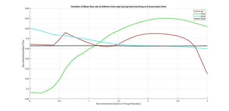
The above graph represents the mass flow at different time steps. However, the mass flow rate reaches the steady-state at the 700th time step for the conservation form.
2. Steady-state distribution of primitive variables inside the nozzle
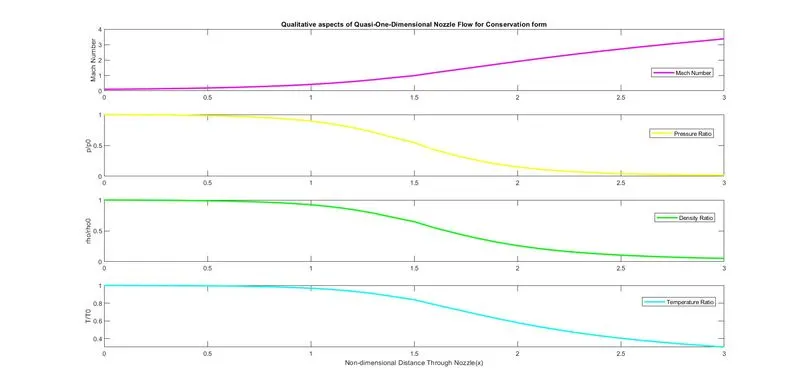
The above quasi-one-dimensional nozzle flow of the Conservative form shows that the primitive variables like Density, Temperature, Pressure, and Mach number from subsonic to supersonic through nozzle distance.
3. Time-wise variation of primitive variables
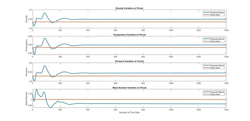
The above graph is a comparison of the Numerical results and Exact results of The Time-wise variation of the Density, Temperature, Pressure, and Mach number at the nozzle throat through the different time steps.
Main Program:-
clear all
close all
clc

% Inputs
n = 31;
x = linspace(0,3,n);
dx = x(2)-x(1);
gamma = 1.4;
throat = (n+1)/2;

% Area
a = 1 + 2.2*(x - 1.5).^2;

% Non-Conservtive form
tic
[rho, t, v, nt, dt, k, mass_flow, pressure, Mach, rho_th, v_th, t_th, pressure_th, Mach_th, M_exact, p_exact, rho_exact, t_exact] = non_conservative_form(n,x,dx,gamma,throat,a);
Non_conservation_time = toc;

% Conservative form
tic
[nt_c, dt_c, l, rho_c, t_c, v_c, mass_flow_c, pressure_c, Mach_c, rho_c_th, v_c_th, t_c_th, pressure_c_th, Mach_c_th] = conservative_form(n,x,dx,gamma,throat,a);
Conservation_time = toc;

% grid dependence test
Forms = {'Exact_value'; 'Non-Conservation form'; 'Conservation form'};
Density = [0.634; rho(throat); rho_c(throat)];
Temperature = [0.833; t(throat); t_c(throat)];
Pressure = [0.528; pressure(throat); pressure_c(throat)];
Mach_number = [1.000; Mach(throat); Mach_c(throat)];
T = table(Forms, Density, Temperature, Pressure, Mach_number);

% comparision of steady-state mass flow variation of both forms
figure(7)
plot(x,mass_flow,'m','linewidth',2)
hold on
plot(x,mass_flow_c,'c','linewidth',2)
xlabel('x/L')
ylabel('Nondimensional Mass Flow rate')
legend('Non-Conservation Form','Conservation Form')
text1 = sprintf('Non-conservation Time = %fs',Non_conservation_time);
text2 = sprintf('Conservation Time = %f s',Conservation_time);
title({'Comparision of Normalized Mass Flow rate Distributions';text1;text2})
1. Comparison of Normalized mass flow rate distributions of both forms:-
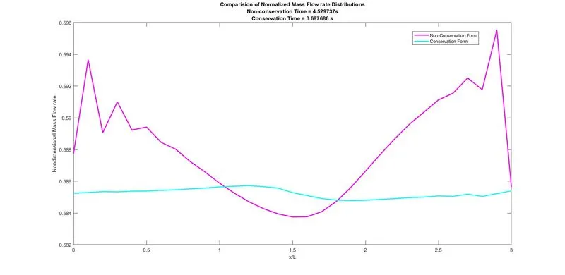
2. Grid dependence test:-

Result & Conclusion:-
- The conservation form yields a better mass flow distribution. The conservation form simply does a better job of conserving mass.
- The non-conservation forms produce slightly more accurate results for the primitive variables, and the conservation forms produce slightly more accurate results for the flux variables. The result for both forms is satisfactory.
- The Solution of the conservation form requires marginally more work. Due to the need to decode the primitive variables from the flux variables, such decoding is not necessary to solving the non-conservation form.
- As a result, the Conservation form is faster(3.697686 seconds) than the Non-Conservation form(4.529737 seconds).