Week 5.1 - Mid term project - Solving the steady and unsteady 2D heat conduction problem

Steady and Unsteady 2D Heat Conduction Problem.

Steady State Analysis

Steady State 2D Heat Conduction Equation

`(∂^2T)/(Δx^2) + (∂^2T)/(Δy^2) = 0`

To Discretize the equation by Central Differncing Scheme

`(∂^2T)/(Δx^2) = (T_L - 2*T_P + T_R) / (Δx^2)`

`(∂^2T) / (Δy^2) = (T_T - 2*T_P + T_B) / (Δy^2)`

`(T_L - 2*T_P + T_R) / (Δx^2) + (T_T - 2*T_P + T_B) / (Δy^2) = 0`

Taking the common terms to LHS

`(2*T_P) / (Δx^2) + (2.T_P) / (∂Δ^2) = (T_L + T_R) / (Δx^2) + (T_T+T_B) / (Δy^2)`

`T_P(2*(∂x^2 +∂y^2)/(Δx^2*Δy^2)) = (T_L +T_R)/(Δx^2) + (T_T+T_B)/(Δy^2`

Assume K = `2* (1/(Δx^2) +1/(Δy^2))`

`T_P. K = (T_L +T_R)/(∂x^2) + (T_T +T_B)/(∂y^2)`

`T_P = (1/K)*((T_L+T_R)/(Δx^2) + (T_T+ T_B)/(Δy^2))`

The above equation is used in the 3 iterative methods

Jacobi Method

`(T_P)^(n+1) = (1/K)*[(T_L+T_R)/(Δx^2) + (T_T+ T_B)/(Δy^2)]^n`

Gauss Seidel Method

`(T_P)^(n+1) = (1/K)*[(T_L+T_R)/(Δx^2) + (T_T+ T_B)/(Δy^2)]^(n+1)`

Sucessive Over-Relaxation Method

`(T_P)^(n+1) = (1-alpha) *(T_P)^n + alpha *((T_L+T_R)/(Δx^2) + (T_T+ T_B)/(Δy^2))`

where,

α is the Sucessive Over-Relaxation Factor

α = 1.1

Steady State 2D Heat Conduction Analysis Using Matlab

% Code to solve steady state equation

close all
clear all
clc

% Inputs
nx = 10;
ny = nx;
L = 1;
alpha = 1.1;

% Assigning Boundary condition
T = ones(nx,ny);
T(:,1) = 400; % Left
T(:,end) = 800; % Right
T(1,:) = 600; % Top
T(end,:) = 900; % Bottom

% Taking average for cornor boundary
T(1,1) = (600 + 400)/2;
T(1,end) = (600 + 800)/2;
T(end,1) = (900 + 400)/2;
T(end,end) = (900 + 800)/2;

% Calculation
x = linspace(0,L,nx);
dx = L/(nx-1);
y = linspace(0,L,ny);
dy = L/(ny-1);

% Assumption
k = (2*(dx^2+dy^2)/(dx^2*dy^2));

T_old = T;
error = 9e9;
tolerance = 1e-4;

% Steady State Analysis
for iterative_solver = [1 2 3]
    if iterative_solver == 1
       T_jacobi = jacobi(x, y, dx, dy, nx, ny, T, k);
    end
    
    if iterative_solver == 2
        T_gauss_seidel = gauss_seidel(x, y, dx, dy, nx, ny, T, k);
    end
    
    if iterative_solver == 3
        T_sor = sor(x, y, dx, dy, nx, ny, T, k);
    end
end

Function Code for Jacobi Method

function [out] = jacobi(x, y, dx, dy, nx, ny, T, k)
% Jacobi method

meshgrid(x,y)

T_old = T;
jacobi_iter = 1;
error = 9e9;
tolerance = 1e-4;

tic
    while(error > tolerance)
        for i = 2:nx-1
            for j = 2:ny-1
                term_1 = (T_old(i-1,j) + T_old(i+1,j))/(k*(dx^2));
                term_2 = (T_old(i,j-1) + T_old(i,j+1))/(k*(dy^2));
                T(i,j) = term_1 + term_2;
            end
        end
        error = max(max(abs(T_old - T)));
        T_old = T;
        jacobi_iter = jacobi_iter + 1;

    end
    iteration_time = toc;
        
    figure(1)
    [a, b] = contourf(x, y, T);
    colormap(jet)
    clabel(a, b)
    colorbar
    xlabel('x axis')
    ylabel('y axis')
    set(gca,'YDIR','reverse')
    text1 = sprintf('Jacobi Iteration Number = %d', jacobi_iter);
    text2 = sprintf('Jacobi Simulation Runtime = %f s', iteration_time);
    title({'Steady State Analysis'; text1; text2})
    pause(0.03)
       
    out = iteration_time;

end

Function Code for Gauss Seidel Method

function [out] = gauss_seidel(x, y, dx, dy, nx, ny, T, k)
% Gauss Seidel Method

meshgrid(x,y)

T_old = T;
gauss_seidel_iter = 1;
error = 9e9;
tolerance = 1e-4;

tic
    while (error > tolerance)
        for i = 2:nx-1
            for j = 2:ny-1
                term_1 = (T(i-1,j) + T_old(i+1,j))/(k*(dx^2));
                term_2 = (T(i,j-1) + T_old(i,j+1))/(k*(dy^2));
                T(i,j) = term_1 + term_2;
            end
        end
        error = max(max(abs(T_old - T)));
        T_old = T;
        gauss_seidel_iter = gauss_seidel_iter + 1;
        
    end
    iteration_time = toc;
       
    figure(2)
    [a, b] = contourf(x, y, T);
    colormap(jet)
    clabel(a, b)
    colorbar
    xlabel('x axis')
    ylabel('y axis')
    set(gca,'YDIR','reverse')
    text1 = sprintf('Gauss Seidel Iteration Number = %d', gauss_seidel_iter);
    text2 = sprintf('Gauss Seidel Simulation Runtime = %f s', iteration_time);
    title({'Steady State Analysis'; text1;text2})
    pause(0.03)
        
    out = iteration_time;
end

Function Code for Sucessive Over-relaxation Method

function [out] = sor(x, y, dx, dy, nx, ny, T, k)
% Successive over-relaxation Method

meshgrid(x,y)

T_old = T;
alpha = 1.1;
sor_iter = 1;
error = 9e9;
tolerance = 1e-4;

tic
    while(error > tolerance)
        for i = 2:nx-1
            for j = 2:ny-1
                term_1 = (T(i-1,j) + T(i+1,j))/(k*(dx^2));
                term_2 = (T(i,j-1) + T(i,j+1))/(k*(dy^2));
                T(i,j) = (1-alpha)*T_old(i,j) + alpha*(term_1 + term_2);
            end
        end
        error = max(max(abs(T_old - T)));
        T_old = T;
        sor_iter = sor_iter + 1;
        
    end
    iteration_time = toc;

    figure(3)
    [a, b] = contourf(x, y, T);
    colormap(jet)
    clabel(a, b)
    colorbar
    xlabel('x axis')
    ylabel('y axis')
    set(gca,'YDIR','reverse')
    text1 = sprintf('SOR Iteration Number = %d', sor_iter);
    text2 = sprintf('SOR Simulation Runtime = %f s', iteration_time);
    title({'Steady State Analysis'; text1;text2})
    pause(0.03)

    out = iteration_time;
end

Plot Result:

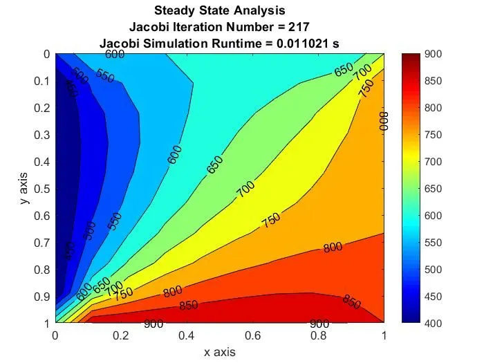
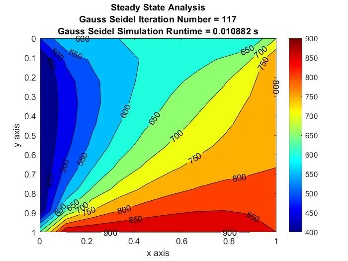
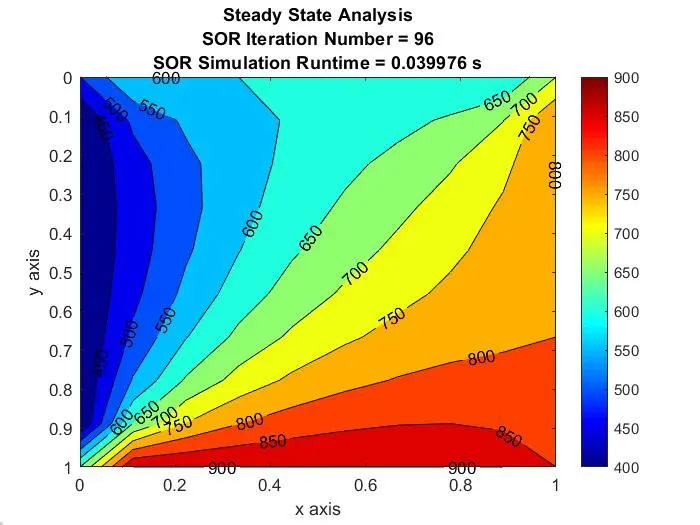
From the ploted graph ,the Sucessive Over-Relaxation method is more effective. The Number of Iteration and Simulation Runtime is very low compared to the other two methods Jacobi and Gauss Seidel. so the optimum value should be obtained from SOR method. The Alpha value is 1.1.

Unsteady/Transient State Analysis.

Transient state 2D Heat Conduction Equation

`(∂T)/(∂t)-α((∂^2T)/(Δx^2) + (∂^2T)/(Δy^2))= 0`

`(T_P^(n+1) - T_P^(n))/(Δt) - alpha ((∂^2T)/(Δx^2) + (∂^2T)/(Δy^2)) = 0`

By Applying Central differencing Scheme

`(T_P^(n+1) - T_P^(n))/(Δt) - alpha*((T_L - 2*T_P + T_R) / (Δx^2) + (T_T - 2*T_P + T_B) / (Δy^2)) = 0`

`T_P^(n+1) = T_P^(n)+ Δt*alpha*((T_L - 2*T_P + T_R) / (Δx^2) + (T_T - 2*T_P + T_B) / (Δy^2))`

Assume `k1 = (alpha*Deltat)/ (Deltax^2)`

`k2 = (alpha*Deltat)/ (Deltay^2)`

If CFL < 0.5 solution is stable

CFL > 0.5 is Unstable ( Solution is wrong)

Then we get

`T_P^(n+1) = T_P^(n)+ k1*(T_L - 2*T_P + T_R) + k2* (T_T - 2*T_P + T_B)`

The above equation are used in both Implicit and Explicit method

Implicit method

Jacobi Method

`T_P^(n+1) = ((1)/(1+2*k1+2*k2))*[T_P^(n)+ k1*(T_L^n + T_R^n) + k2* (T_T^n + T_B^n)]`

Gauss Seidel Method

`T_P^(n+1) = ((1)/(1+2*k1+2*k2))*[T_P^(n)+ k1*(T_L + T_R) + k2* (T_T + T_B)]`

Sucessive Over-Relaxation factor

`T_P^(n+1) =[(1 - omega) * T_P^n] + omega * [((1)/(1+2*k1+2*k2))*[T_P^(n)+ k1*(T_L + T_R) + k2* (T_T + T_B)]]`

where,

ω is the Sucessive over-Relaxation factor = 1.1

Transient State 2D Heat Conduction Analysis for Implicit Method Using Matlab

% Code to solve Transient State Equation

close all
clear all
clc

% Inputs
nx = 10;
ny = nx;
L = 1;
t = 1.5;
dt = 0.01;
nt = t/dt;
alpha = 1.5;

% Assigning Boundary condition
T = ones(nx,ny);
T(:,1) = 400; % Left
T(:,end) = 800; % Right
T(1,:) = 600; % Top
T(end,:) = 900; % Bottom

% Taking average for corner boundary
T(1,1) = (600 + 400)/2;
T(1,end) = (600 + 800)/2;
T(end,1) = (900 + 400)/2;
T(end,end) = (900 + 800)/2;

% Calculation
x = linspace(0,L,nx);
dx = L/(nx-1);
y = linspace(0,L,ny);
dy = L/(ny-1);

% Assumption
k1 = alpha*(dt/dx^2);
k2 = alpha*(dt/dy^2);

T_old = T;
error = 9e9;
tolerance = 1e-4;

% Transient State Analysis by Implicit Method


for iterative_solver = [1 2 3]
    if iterative_solver == 1
        T_jacobi = implicit_jacobi(x, y, nx, ny, T, t, dt, k1, k2);
    end
    
    if iterative_solver == 2
        T_gauss_seidel = implicit_gauss_seidel(x, y, nx, ny, T, t, dt, k1, k2);
    end
    
    if iterative_solver == 3
        T_sor = implicit_sor(x, y, nx, ny, T, t, dt, k1, k2);
    end
end

Function code for Implicit Jacobi Method:

function [out] = implicit_jacobi(x, y, nx, ny, T, t, dt, k1, k2)
% Implicit Jacobi Method

meshgrid(x,y)

T_old = T;
T_prev = T;
jacobi_iter = 1;
nt = t/dt;
error = 9e9;
tolerance = 1e-4;

tic
% Time Loop
    for k = 1:nt
        % Convergence Loop
        while(error > tolerance)
            % Space Loop
            for i = 2:nx-1
                for j = 2:ny-1
                    term_1 = (1+(2*k1)+(2*k2))^-1;
                    term_2 = k1*term_1;
                    term_3 = k2*term_2;
                    H = (T_old(i-1,j) + T_old(i+1,j));
                    V = (T_old(i,j-1) + T_old(i,j+1));
                    T(i,j) = (term_1*T_prev(i,j)) + (H*term_2) + (V*term_3); 
                end
            end
            error = max(max(abs(T_old - T)));
            T_old = T;
            jacobi_iter = jacobi_iter + 1;

        end
        T_prev = T;           
        
    end
    iteration_time = toc;
    
    figure(4)
    [a, b] = contourf(x, y, T);
    colormap(jet)
    clabel(a, b)
    colorbar
    xlabel('x axis')
    ylabel('y axis')
    set(gca,'YDIR','reverse')
    text1 = sprintf('Implicit Jacobi Iteration number = %d', jacobi_iter);
    text2 = sprintf('Implicit Jacobi Simulation Runtime = %f s', iteration_time);
    title({'Transient State Analysis'; text1; text2})
    pause(0.03)
    
    out = iteration_time;
end

Function code for Implicit Gauss Seidel Method:

function [out] =  implicit_gauss_seidel(x, y, nx, ny, T, t, dt, k1, k2)
%Implicit Gauss Seidel Method

meshgrid(x,y)

T_old = T;
T_prev = T;
gauss_seidel_iter = 1;
nt = t/dt;
error = 9e9;
tolerance = 1e-4;

tic
% Time Loop
    for k = 1:nt
        % Convergence Loop
        while(error > tolerance)
            % Space Loop
            for i = 2:nx-1
                for j = 2:ny-1
                    term_1 = (1+(2*k1)+(2*k2))^-1;
                    term_2 = k1*term_1;
                    term_3 = k2*term_2;
                    H = (T(i-1,j) + T(i+1,j));
                    V = (T(i,j-1) + T(i,j+1));
                    T(i,j) = (term_1*T_prev(i,j)) + (H*term_2) + (V*term_3);
                end
            end
            error = max(max(abs(T_old - T)));
            T_old = T;
            gauss_seidel_iter = gauss_seidel_iter + 1;
            
            
        end
        T_prev = T;   
        
    end
    iteration_time = toc;
    
    figure(5)
    [a, b] = contourf(x, y, T);
    colormap(jet)
    clabel(a, b)
    colorbar
    xlabel('x axis')
    ylabel('y axis')
    set(gca,'YDIR','reverse')
    text1 = sprintf('Implicit Gauss Seidel Iteration number = %d', gauss_seidel_iter);
    text2 = sprintf('Implicit Gauss Seidel Simulation Runtime = %f s', iteration_time);
    title({'Transient State Analysis'; text1; text2})
    pause(0.03)
    
    out = iteration_time;
end

Function code for Implicit Sucessive Over-relaxation Method:

function [out] = implicit_sor(x, y, nx, ny, T, t, dt, k1, k2)
% Implicit Successive over-relaxation Method

meshgrid(x,y)

T_old = T;
T_prev = T;
sor_iter = 1;
nt = t/dt;
omega = 1.1;
error = 9e9;
tolerance = 1e-4;

tic
% Time Loop
    for k = 1:nt
        % Convergence Loop
        while(error > tolerance)
            % Space Loop
            for i = 2:nx-1
                for j = 2:ny-1
                    term_1 = (1+(2*k1)+(2*k2))^-1;
                    term_2 = k1*term_1;
                    term_3 = k2*term_2;
                    H = (T(i-1,j) + T(i+1,j));
                    V = (T(i,j-1) + T(i,j+1));
                    T(i,j) = (1-omega)*T_old(i,j) + omega*(term_1*T_prev(i,j)) + (H*term_2) + (V*term_3);
                end
            end
            error = max(max(abs(T_old - T)));
            T_old = T;
            sor_iter = sor_iter + 1;
            
        end
        T_prev = T;        
        
    end
    iteration_time = toc;
    
    figure(6)
    [a, b] = contourf(x, y, T);
    colormap(jet)
    clabel(a, b)
    colorbar
    xlabel('x axis')
    ylabel('y axis')
    set(gca,'YDIR','reverse')
    text1 = sprintf('Implicit SOR Iteration number = %d', sor_iter);
    text2 = sprintf('Implicit SOR Simulation Runtime = %f s', iteration_time);
    title({'Transient State Analysis'; text1; text2})
    pause(0.03)
    
    out = iteration_time;
end
        

Plot Result:

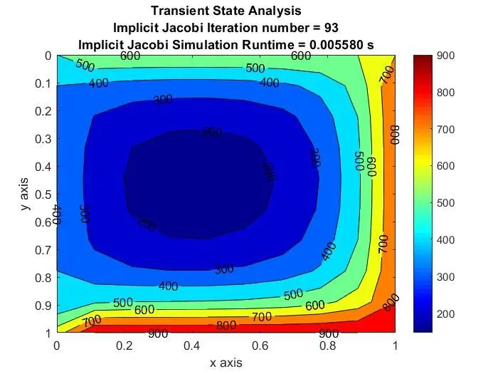
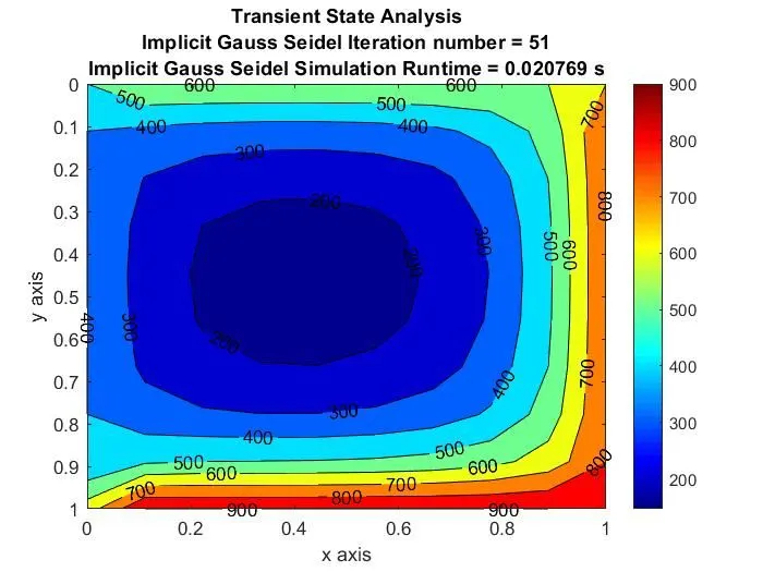
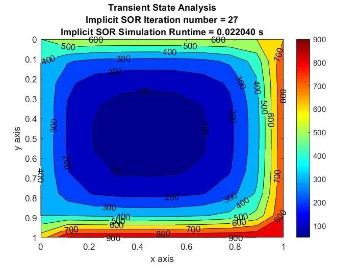
From the plotted graph, the Successive Over-Relaxation method is more effective. The Number of Iteration and Simulation Runtime is very low compared to the other two methods Jacobi and Gauss-Seidel. The relaxation factor ω = 1.1 and the Thermal Diffusivity α = 1.5. Therefore the optimum value should be obtained from the SOR method.

Explicit Method

`T_P^(n+1) = (1- (2*k1) - (2*k2))*T_P^(n)+[ k1*(T_L^n + T_R^n) + k2* (T_T^n + T_B^n)]`

Transient State 2D Heat Conduction Analysis for Explicit Method Using Matlab

% Code to solve Transient State Equation

close all
clear all
clc

% Inputs
nx = 10;
ny = nx;
L = 1;
t = 1.4;
dt = 1e-3;
nt = t/dt;
alpha = 1.5;

% Assigning Boundary condition
T = ones(nx,ny);
T(:,1) = 400; % Left
T(:,end) = 800; % Right
T(1,:) = 600; % Top
T(end,:) = 900; % Bottom

% Taking average for corner boundary
T(1,1) = (600 + 400)/2;
T(1,end) = (600 + 800)/2;
T(end,1) = (900 + 400)/2;
T(end,end) = (900 + 800)/2;

% Calculation
x = linspace(0,L,nx);
dx = L/(nx-1);
y = linspace(0,L,ny);
dy = L/(ny-1);

% Assumption
k1 = alpha*(dt/dx^2);
k2 = alpha*(dt/dy^2);

T_old = T;
error = 9e9;
tolerance = 1e-4;

% Transient State Analysis by Explicit Method
iterative_solver = 1;

tic
if iterative_solver == 1
    solver = 1;
    while (error > tolerance)
        for i = 2:nx-1
            for j = 2:ny-1
                term_1 = (T_old(i-1,j) + T_old(i+1,j));
                term_2 = (T_old(i,j-1) + T_old(i,j+1));
                T(i,j) = ((1- 2*k1- 2*k2)*T_old(i,j)) + (k1*term_1) + (k2*term_2);
            end
        end
        error = max(max(abs(T_old -T)));
        T_old = T;
        solver = solver + 1;
    end
end
time = toc;

figure(7)
[a, b] = contourf(x, y, T);
colormap(jet)
clabel(a, b)
colorbar
xlabel('x axis')
ylabel('y axis')
set(gca,'YDIR','reverse')
text1 = sprintf('Transient Explicit Iteration number = %d', solver);
text2 = sprintf('Transient Explicit Simulation Runtime = %f s', time);
title({'Transient State Analysis'; text1; text2})

Plot Result:

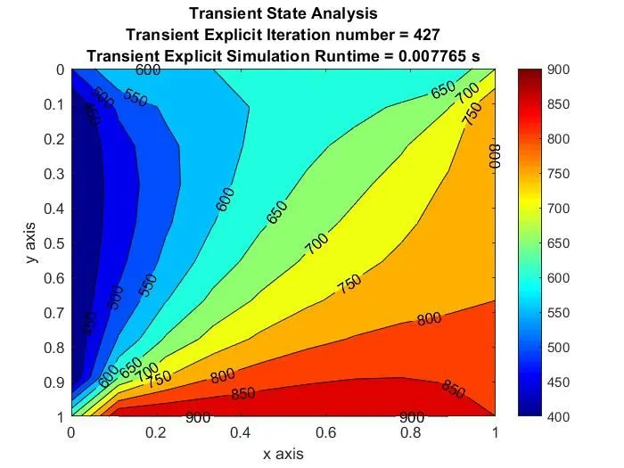
The Transient State for Explicit method should be analysed. The SOR method depends upon the factor like thermal diffusion, relaxation factor and CFL. To change these factor and easily finf the accurate and optimum Solution.