Week 9 - FVM Literature Review

FVM Literature Review

1. Finite Volume Method (FVM):-

       The Finite Volume Method (FVM) is a discretization method for the approximation of a single or a system of partial differential equations expressing the conservation, or balance, of one or more quantities. These partial differential equations (PDEs) are often called conservation laws, they may be of different nature, eg. biophysics, chemistry, image processing, finance, dynamic reliability. These describe the relations between partial derivatives of unknown fields such as temperature, concentration, pressure, molar fraction, the density of electrons, or probability density function, with respect to variables within the domain under consideration.

As in the finite element method, a mesh is constructed, which consists of a partition of the domain where the space variable lives. The elements of the mesh are called control volumes. The integration of the PDE over each control volume results in a balanced equation. The main issue is the discretization of the fluxes at the boundaries of each control volume: in order for the FVM to be efficient, the numerical fluxes are generally

• conservative, the flux entering a control volume from its neighbour must be the opposite of the one entering the neighbour from the control volume,
• consistent, the numerical flux of a regular function interpolation tends to the continuous flux as the mesh size vanishes.

2. Major Difference between FDM & FVM:-

a. Finite difference Method

• The finite-difference method is the most direct approach to discretizing partial differential equations. 
• The finite-difference method is typically defined on a regular grid and this fact can be used for very efficient solution methods.
• The method is therefore not usually used for irregular CAD geometries, but more often for rectangular or block-shaped models.
• Certain formulations of the finite-element method defined on a regular grid are identical to a finite-difference method on the same grid.
• Regular grids can often be used in metrological, seismological, and astrophysical simulations.

b. Finite Volume Method

• The Finite-volume method is similar to the finite-element method in that the CAD model is first divided into very small but finite-sized elements of geometrically simple shapes.
• The finite-volume method is very different from the finite-element method, beginning with the concept of elements, which are instead referred to as cells.
• The finite-volume method is based on the fact that many physical laws are conservation laws - what goes into one cell on one side needs to leave the same cell on another side.
• This method has been very successful in solving fluid flow problems.

 3. Need for Interpolation schemes and Flux Limiters.

      The nature of the transport equations governing fluid flow and heat transfer and the formal control volume integration. The numerical method based on this integration, the finite volume method considering the simplest transport process of all pure diffusion in the steady-state.

Considering 1D Heat conduction equation.  

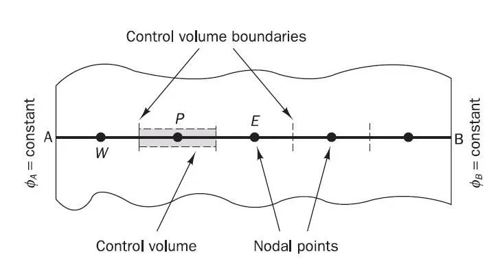
The governing equation is 

`d/dx(alpha.(dT)/dx) + S = 0`

where,

`alpha`=  Function of Temperature

S = source term

The Intergral form of governing equation is 

`int(∂/(∂x) (alpha.(∂T)/(∂x)) +S) dv = 0`

 

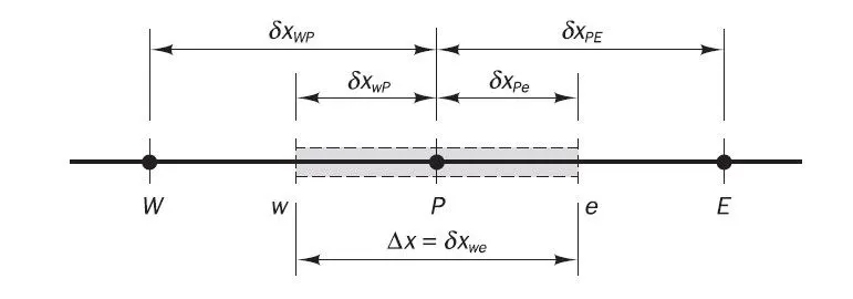
 To discretize the finite volume method is the integration of the governing equation over a control volume to yield a discretized equation at its nodal point P.

`int(∂/(∂x) (alpha. (∂T)/(∂x)) A.dx + int(S.dv) = 0`

`[alpha.A.(∂T)/(∂x)]_e - [alpha.A.(∂T)/(∂x)]_w + barS.dv = 0`

Here, 

A = Face volume of area

dv = Volume

`barS`= Average value of source(S) over the control volume.

 For the Diffusive heat flux terms are,

`alpha.A[(T_E-T_p)/(Deltax)]-alpha.A[(T_P-T_W)/(Deltax)] +barS.dv = 0`

The source term is a function of the dependent variable. In such cases the finite volume method approximation the source term by means of a linear form

`barS.dv = S_u +S_P.T_P`

`alpha.A[(T_E-T_p)/(Deltax)]-alpha.A[(T_P-T_W)/(Deltax)] +(S_u+S_P.T_P) = 0`

Hence the equation says that the,

`[Heatflux]_("out") -[Heatflux]_("in") +Sourceterm = 0`

The amount of heat that is removed from a particular box is conserved.

Gradient Scheme:-

   To evaluate the numerically represent the gradient of temperature from which point should use the information and how could the scheme should be structure. That is called a gradient scheme.

Interpolation Schemes:-

• The surface integral and the volume integrals in the finite volume formulation. They require values at locations other than the computational nodes of the control volume.
• The value at this location is obtained by the interpolation formula.
• Hence the interpolation schemes are important in the finite-volume method.

There are various types of interpolation methods in FVM.

1. Upwind interpolation scheme

2. Linear interpolation scheme

3. Quadratic Upwind interpolation scheme

4. Hybrid interpolation scheme

5. Total Variation Diminishing (TVD) scheme

1. Upwind interpolation scheme:-

• The upwind interpolation scheme for approximating the value of a variable f at the east face of a control volume is 

       `f_e = {(f_p if (v.n)_e > 0) ,(f_E if (v.n)_e < 0):}`

• The upwind differencing scheme utilizes consistent expressions to calculate fluxes through cell faces: therefore it can be easily shown that the formulation is conservative.
• The coefficients of the discretized equation are always positive and satisfy the requirements for boundedness. All the coefficients are positive and the coefficient matrix is diagonally dominant, hence no 'wiggles' occur in the solution.
• The scheme is based on the backward differencing formula so the accuracy is only first-order on the basis of the Taylor series truncation error.

 2. Linear interpolation scheme:-

• Linear interpolation is the method of generating new data points with a range of a discrete set of known data points.

      `f_e = f_e lamda_e +f_p(1 - lamda_e)`

       where,

      `lamda_e = ((x_e -x_p)/(x_E-x_p))`

• The linear interpolation scheme is the same as the central difference formula that we considered for the first-order derivative. So this scheme is also known as the central differencing scheme.
• Generally, it is used to solve the integration convection-diffusion equation

3. Quadratic Upwind interpolation scheme:-

• The scheme uses consistent quadratic profiles - the cell face values of fluxes are always calculated by quadratic interpolation between two bracketing nodes and an upstream node - and is therefore conservative.
• The transportiveness property is built into the scheme as the quadratic function based on two upstream and one downstream nodal values.
• If the flow field satisfies continuity the coefficient `a_p` equals the sum of all neighbour coefficient, which is desirable for boundedness.
• If `u_w > 0` and `u_e > 0` the east coefficient becomes negative at relatively modest cell Peclet numbers (`Pe_e = (F_e)/(D_e > 8/3)`). 
• This gives rise to stability problems and unbounded solution under certain flow conditions.
• Similarly, the west coefficient can become negative when the flow is in the negative direction. The QUICK scheme is therefore conditionally stable.

4. Hybrid interpolation scheme:-

• The hybrid differencing scheme exploits the favourable properties of the upwind and central differencing schemes. It switches to upwind differencing when central differencing produces an inaccurate result at high Pe numbers.
• The scheme is fully conservative and since the coefficient is always positive it is unconditionally bounded.
• The scheme produces a physically realistic solution and is highly stable when compared with higher-order schemes such as QUICK. 
• Hybrid differencing has been widely used in various CFD procedures and has proved to be very useful for predicting practical flows.
• The disadvantage is that the accuracy in terms of Taylor series truncation error is the only first-order.

5. Total Variation Diminishing scheme:-

• TVD schemes are generalisations of existing discretisation scheme, so they inherently satisfy all the necessary requirements of transportiveness, conservativeness and boundedness.
• `f_e = f_p +1/2 psi (r)(f_E -f_p)`

          where `psi` is the flux limiter.

FLUX LIMITERS:-

The Flux limiters are used in high-resolution schemes, to avoid the spurious oscillations (wiggles) that would otherwise occur with high order spatial discretization schemes due to shocks, discontinuities or sharp changes in the solution domain. 

The use of flux limiters, together with an appropriate high-resolution scheme, make the solution Total Variation Diminishing(TVD).

The Flux limiters are also referred to as slope limiters because they both have the same mathematical form, and both have the effect of limiting the solution gradient near shocks or discontinuities.

`F(u_i +1/2) = f_(i +1/2)^(low) - phi(ri)(f_(i+1/2)^(low) - f_(i+1/2)^(high))`

`F(u_i -1/2) = f_ (i-1/2)^(low) - phi(r_i-1) (f_(i -1/2)^(low) - f_(i-1/2)^(high))`

where,

`f^(low)` = low resolution flux,

`f^(high)` = high resolution flux,

`phi(r)` = flux limiter function,

and `r` represents the ratio of successive gradients on the solution mesh,

`r_i = (u_i - u_(i-1))/(u_(i+1) - u_i)`

The limiter function is constrained to be greater than or equal to zero `phi(r)>= 0`. Therefore, when the limiter is equal to zero the flux is represented by a low-resolution scheme. Similarly, when the limiter is equal to 1 it is represented by a high-resolution scheme.