Week 3.5 - Deriving 4th order approximation of a 2nd order derivative using Taylor Table method
Deriving the 4th Order approximation of a 2nd Order derivative using taylor table method.
1. Central difference scheme:-
Number of Nodes(N) = order of derivative(P) + order of approximation(Q) - 1
(N) = 2+4-1
(N) = 5
Hypothesis function for central difference scheme,
`(d^2u)/(dx^2) = af(i-2) + bf(i-1) + cf(i) + df(i+1) + ef(i+2)`
| Stensils | f(i) | Δ(x)*f'(i) | Δ(x)^2*f''(i) | Δ(x)^3*f'''(i) | Δ(x)^4*f''''(i) |
| af(i-2) | a | -2a | 4a/2 | -8a/6 | 16a/24 |
| bf(i-1) | b | -b | b/2 | -b/6 | b/24 |
| cf(i) | c | 0 | 0 | 0 | 0 |
| df(i+1) | d | d | d/2 | d/6 | d/24 |
| ef(i+2) | e | 2e | 4e/2 | 8e/24 | 16e/24 |
| 0 | 0 | 1 | 0 | 0 |
The all unknowns for the central difference are,
close all
clear all
clc

% Central differncing scheme
A = [1 1 1 1 1;
    -2 -1 0 1 2;
    4/2 1/2 0 1/2 4/2;
    -8/6 -1/6 0 1/6 8/6;
    16/24 1/24 0 1/24 16/24];

B = [0;0;1;0;0];

X = rats(linsolve(A,B));
Output:
>> X

X =

  5×14 char array

    '     -1/12    '
    '      4/3     '
    '     -5/2     '
    '      4/3     '
    '     -1/12    '
2. Skewed Right-Sided Difference scheme:-
Number of Nodes(N) = order of derivative(P) + order of approximation(Q)
(N) = 2+4
(N) = 6
Hypothesis function for Skewed Right-Sided Difference scheme,
`(d^2u)/(dx^2) = af(i) + bf(i+1) +cf(i+2) + df(i+3) + ef(i+4) + gf(i+5)`
| Stencil | f(i) | Δ(x)*f'(i) | Δ(x)^2*f''(i) | Δ(x)^3*f'''(i) | Δ(x)^4*f''''(i) | Δ(x)^5*f'''''(i) |
| af(i) | a | 0 | 0 | 0 | 0 | 0 |
| bf(i+1) | b | b | b/2 | b/6 | b/24 | b/120 |
| cf(i+2) | c | 2c | 4c/2 | 8c/6 | 16c/24 | 32c/120 |
| df(i+3) | d | 3d | 9d/2 | 27d/6 | 81d/24 | 243d/120 |
| ef(i+4) | e | 4e | 16e/2 | 64e/6 | 256e/24 | 1024e/120 |
| gf(i+5) | g | 5g | 25g/2 | 125g/6 | 625g/24 | 3125g/120 |
| 0 | 0 | 1 | 0 | 0 | 0 |
All unknown for Skewed Right-sided differencing scheme are,
close all
clear all
clc

% Skewed Right-sided differencing Scheme
C = [1 1 1 1 1 1;
    0 1 2 3 4 5;
    0 1/2 4/2 9/2  16/2 25/2;
    0 1/6 8/6 27/6 64/6 125/6;
    0 1/24 16/24 81/24 256/24 625/24;
    0 1/120 32/120 243/120 1024/120 3125/120];

D = [0;0;1;0;0;0];

Y = rats(linsolve(C,D));
Output:
>> Y

Y =

  6×14 char array

    '     15/4     '
    '    -77/6     '
    '    107/6     '
    '      -13     '
    '     61/12    '
    '     -5/6     '

>>
3. Skewed Left-Sided Difference scheme:-
`(d^2u)/(dx^2) = af(i) + bf(i-1) +cf(i-2) + df(i-3) + ef(i-4) + gf(i-5)`
| Stencil | f(i) | Δ(x)*f'(i) | Δ(x)^2*f''(i) | Δ(x)^3*f'''(i) | Δ(x)^4*f''''(i) | Δ(x)^5*f'''''(i) |
| af(i) | a | 0 | 0 | 0 | 0 | 0 |
| bf(i-1) | b | -b | b/2 | -b/6 | b/24 | -b/120 |
| cf(i-2) | c | -2c | 4c/2 | -8c/6 | 16c/24 | -32c/120 |
| df(i-3) | d | -3d | 9d/2 | -27d/6 | 81d/24 | -243d/120 |
| ef(i-4) | e | -4e | 16e/2 | -64e/6 | 256e/24 | -1024e/120 |
| gf(i-5) | g | -5g | 25g/2 | -125g/6 | 625g/24 | -3125g/120 |
| 0 | 0 | 1 | 0 | 0 | 0 |
All unknown for Skewed left-sided differencing scheme are,
close all
clear all
clc

% Skewed left-sided differencing Scheme
E = [1 1 1 1 1 1;
    0 -1 -2 -3 -4 -5;
    0 1/2 4/2 9/2  16/2 25/2;
    0 -1/6 -8/6 -27/6 -64/6 -125/6;
    0 1/24 16/24 81/24 256/24 625/24;
    0 -1/120 -32/120 -243/120 -1024/120 -3125/120];

F = [0;0;1;0;0;0];

Z = rats(linsolve(E,F));
Output:
>> Z

Z =

  6×14 char array

    '     15/4     '
    '    -77/6     '
    '    107/6     '
    '      -13     '
    '     61/12    '
    '     -5/6     '

>>
All the unknown values are form of algebraic equation. The equation are formed up with the matrix to find the unknown values using matlab.
Main Program;
close all
clear all
clc

% Input parameters
x = pi/3;
dx = linspace(pi/4,pi/400,100);

% Analytical function = exp^(x)*cos(x)

analytical_derivative = -2*exp(x)*sin(x);

for i = 1:length(dx)

    % Function at Various nodes point
    a(i)=(exp(x-(5*dx(i)))*cos(x-(5*dx(i))));
    b(i)=(exp(x-(4*dx(i)))*cos(x-(4*dx(i))));
    c(i)=(exp(x-(3*dx(i)))*cos(x-(3*dx(i))));
    d(i)=(exp(x-(2*dx(i)))*cos(x-(2*dx(i))));
    e(i)=(exp(x-dx(i))*cos(x-dx(i)));
    f(i)=(exp(x)*cos(x));
    g(i)=(exp(x+dx(i))*cos(x+dx(i)));
    h(i) = (exp(x+(2*dx(i)))*cos(x+(2*dx(i))));
    j(i) = (exp(x+(3*dx(i)))*cos(x+(3*dx(i))));
    k(i) = (exp(x+(4*dx(i)))*cos(x+(4*dx(i))));
    l(i) = (exp(x+(5*dx(i)))*cos(x+(5*dx(i))));


    % Formula for taylor series functions

    % Forward Differencing Scheme
    FDS(i) = (g(i)-f(i))/(dx(i));

    % Backward Differencing Scheme
    BDS(i) = (f(i)-e(i))/(dx(i));

    % Central Differencing Scheme
    CDS(i) = (-1*(d(i))+16*(e(i))-30*(f(i))+16*(g(i))-1*(h(i)))/(12*(dx(i)^2)); %#ok<*SAGROW>

    % Skewed Left Sided Difference
    Skewed_left(i) = (45*(f(i))-154*(e(i))+214*(d(i))-156*(c(i))+61*(b(i))-10*(a(i)))/(12*(dx(i)^2));

    % Skewed Right Sided Difference
    Skewed_right(i) = (45*(f(i))-154*(g(i))+214*(h(i))-156*(j(i))+61*(k(i))-10*(l(i)))/(12*(dx(i)^2));


   error_FDS(i) = abs(FDS(i) - analytical_derivative);
   error_BDS(i) = abs(BDS(i) - analytical_derivative);
   error_CDS(i) = abs(CDS(i) - analytical_derivative);
   error_LSD(i) = abs(Skewed_left(i) - analytical_derivative);
   error_RSD(i) = abs(Skewed_right(i) - analytical_derivative);


end

figure(1)
grid on

loglog(dx,error_FDS,'linewidth',2,'marker','s');
hold on
loglog(dx,error_BDS,'linewidth',2,'marker','o');
xlabel('dx')
ylabel('Absolute Error')
legend('Forward Difference Scheme','Backward Difference Scheme')
title('FDS Error Vs BDS Error')

figure(2)
grid on

loglog(dx,error_RSD,'linewidth',2,'marker','pentagram');
hold on
loglog(dx,error_LSD,'linewidth',2,'marker','hexagram');
hold on
loglog(dx,error_CDS,'linewidth',2,'marker','d');
xlabel('dx')
ylabel('Absolute Error')
legend('Skewed Right sided Difference of 4th Order','Skewed Left sided Difference of 4th order','Central Difference Scheme of 4th order')
title('Comparison of Different Scheme')
Result:
Ploted graph:-
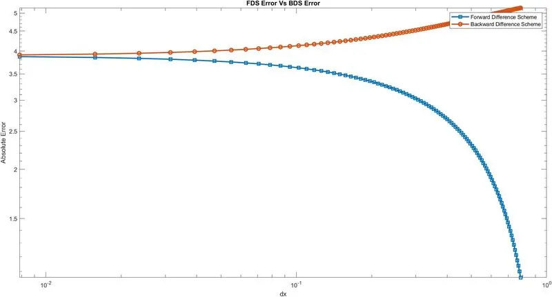
1.Forward differencing Scheme(FDS) Errors vs Backward Differencing Scheme (BDS) Error
2. Comparision of Different scheme.
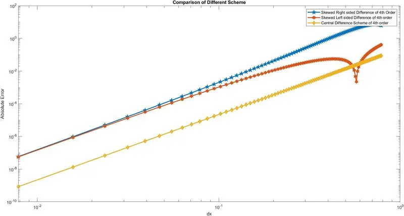
- The Forward Differencing Scheme and Backward Differencing Scheme equation are solve with the 1st order approximation with 1st order derivative and Central Differencing Scheme solve with 2nd order approximation and 1st order derivative. Both are using the same point and CDS provide the accurate result.
- The Output Graph for Central differencing scheme(CDS), skewed Left, skewed right the CDS have less error than the other schemes.
- So, that the CDS gives the accurate result and less error in 4th order approximation of 2nd order derivative.
Why a skewed scheme is useful? What can a skewed scheme do that a Central differencing scheme cannot?
The skewed scheme is provide when the node points are in one side of the grid. For corner node with higher approximation the skewed scheme is used accurate result, central scheme cannot applyed in it. so that the skewed scheme is very useful for one direction.