Parametric study on gate valve

Aim : For this challenge, you will have to perform a parametric study on the gate valve simulation by setting the opening from 10 % to 80%.

Objectives :

1. Obtain the mass flow rates at the outlet for each design point.
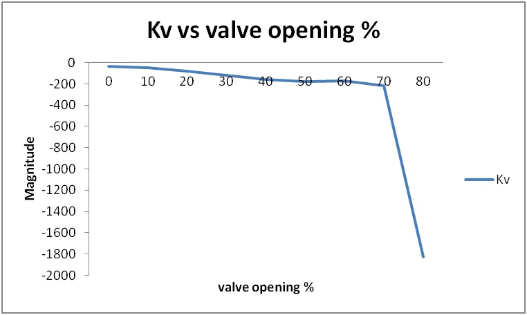
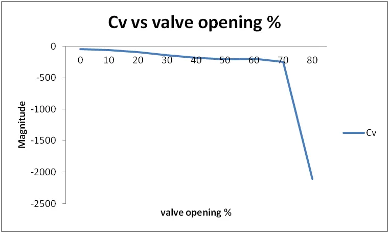
2. Calculate the flow coefficient and flow factor for each opening and plot the graph.
3. Discuss the results of the mass flow rate and flow coefficient.

Submit a well-defined report with all the necessary details.

Theory :

1. Gate valve :

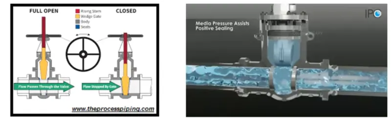
• Gate valves are mainly used in industries to shut the flow of fluid or control the fluid flow.
• They can be found in petrochemical industries, power plants and widely in the pipeline industries.
• The gate valve looks as

2. Parametrizing the lift :

• In this challenge, we are trying to study how our mass flow rate is going to be change w.r.t. change in the gate valve opening position i.e. change of the different lifts of the gate disc, so only change in the case setup will be this geometrical value.
• By parameterizing the lift value, we are essentially automating the meshing, the solution setup and post-processing stages for saving time and it is more efficient.

2.1. Input parameter :

• For the parametric study, the input parameter that needs to be parametrized is the lift of the gate-disc.

2.2. Output parameter :

• For the varying the lifts of the gate disc, we are trying to find out the change it causes in the flow, which can be studied by monitoring the mass flow rate at the outlet.
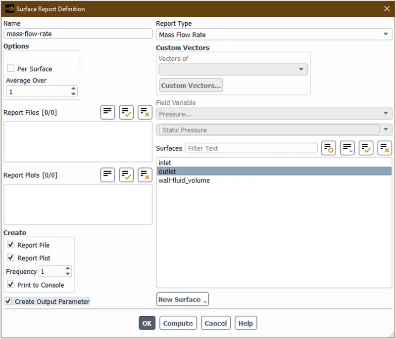
• The mass flow rate is made by report definitions and by enabling the create output parameter; it will be parametrized as well.

3. Flow factor and flow coe. :

• The flow coefficient (Cv) of a device is a relative measure of its efficiency at allowing fluid flow. It describes the relationship between the pressure drop across an orifice valve or other assembly and the corresponding flow rate.

`Q=C_v sqrt((ΔP)/S)`

Where,

Q=rate of flow (US gallons/minute)

S=specific gravity of the fluid (for water, S = 1)

ΔP=pressure drop across the valve (psi).

• The metric equivalent flow factor (Kv) is calculated using metric units

`Q=K_v sqrt((ΔP)/S)`

Where,

Q=rate of flow (m³/h)

S=specific gravity of the fluid (for water, S = 1)

∆P=pressure drop across the valve (bar).

K_v can be calculated from C_v using the equation:

K_v= 0.865C_v

Model approach :

1. Pre-processing methods :

1.1. Geometry :

• Open ansys workbench
• Drag the fluid flow(fluent) to the project scheme
• Open space-claim
• Import the geometry

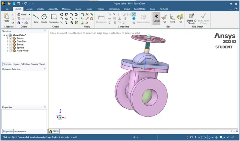
• First of all hide all the parts except gate disc and spindle

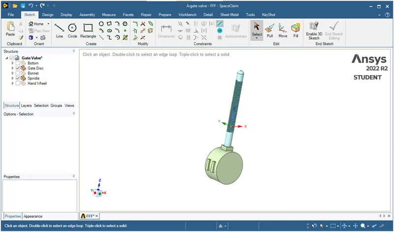
Now click on move

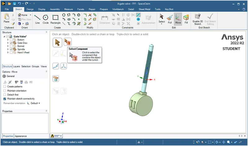
Now click on select component tab and select the total components

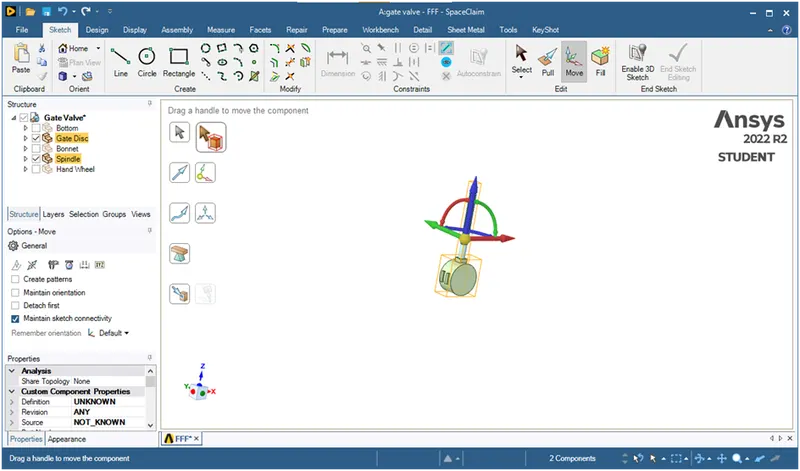
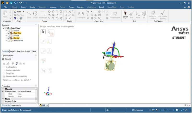
Now just lift it and give dimension as 10mm

Now goto groups -> click on create the parameter

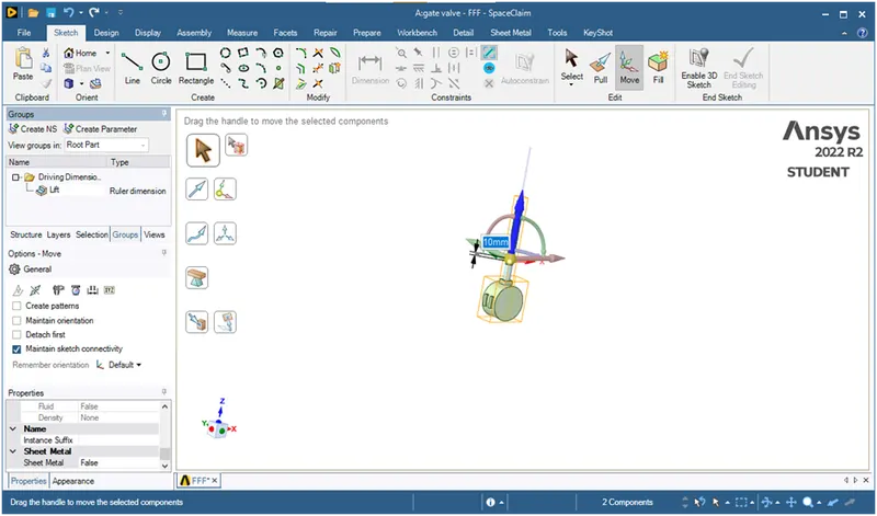
Now its done .

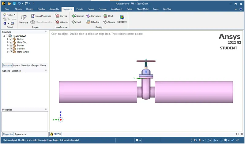
• Now goto structures and show bottom part

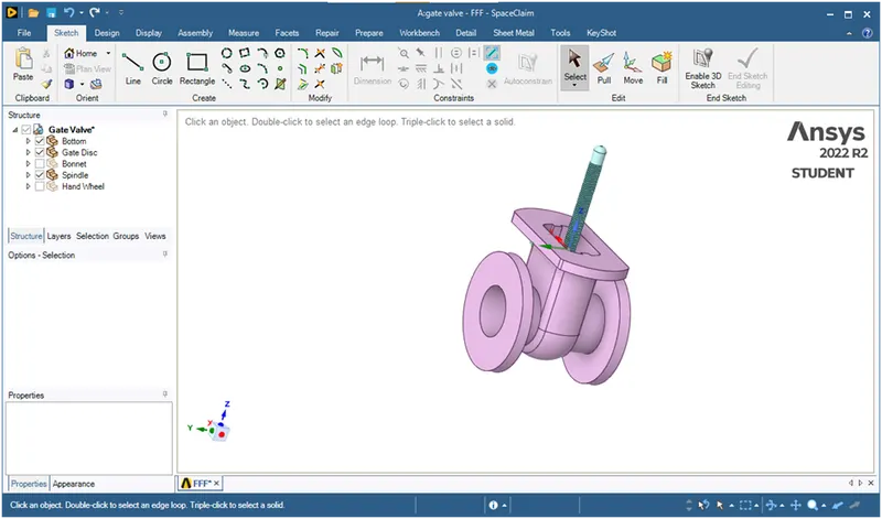
Now pull the surface as shown below

• Now extract the fluid volume by selecting required edges

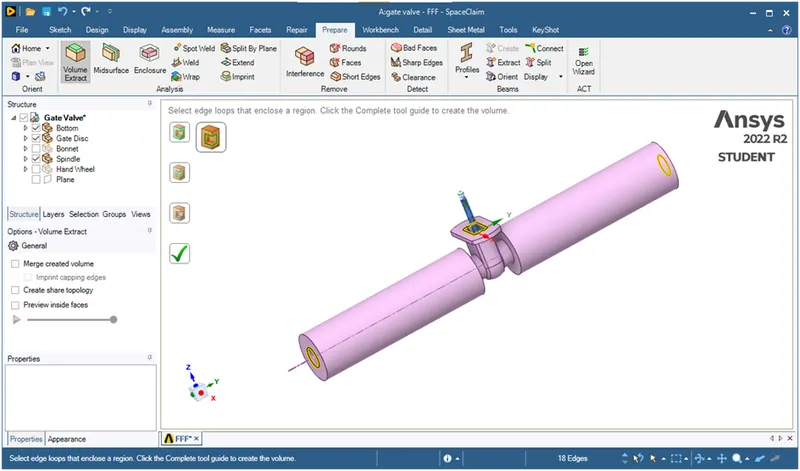
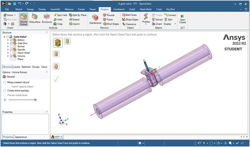
Let see c/s view

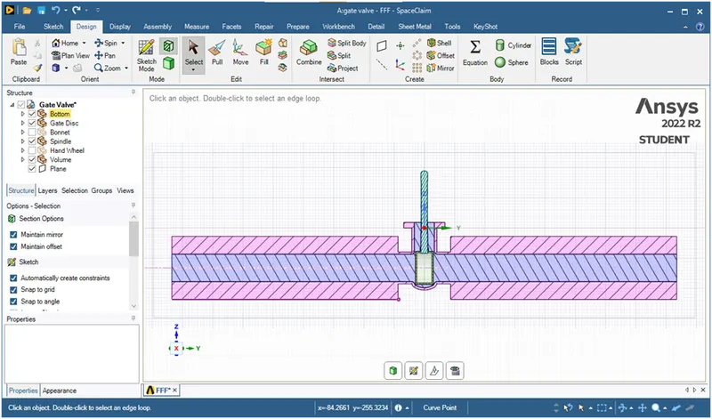
Lets try to change lift as 10 mm and then right click on volume -> update volume by contex

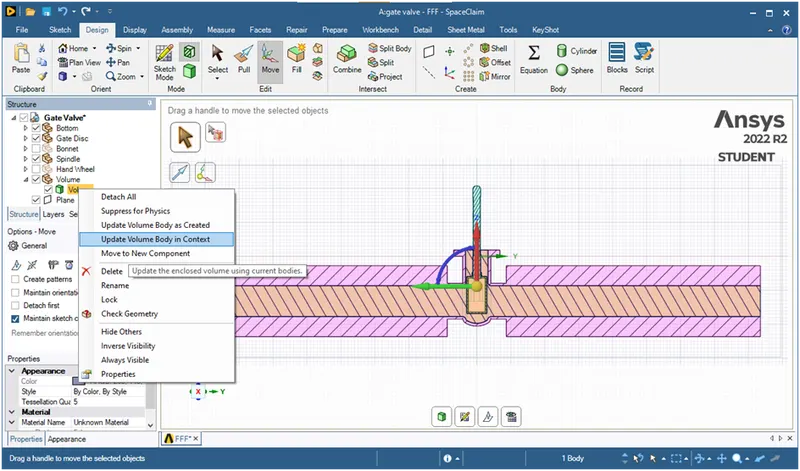
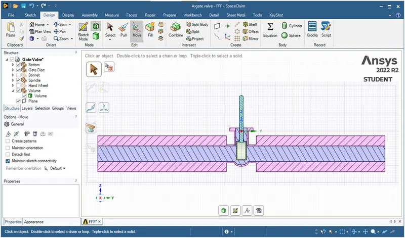
• Now suppress all solid bodies for physics.

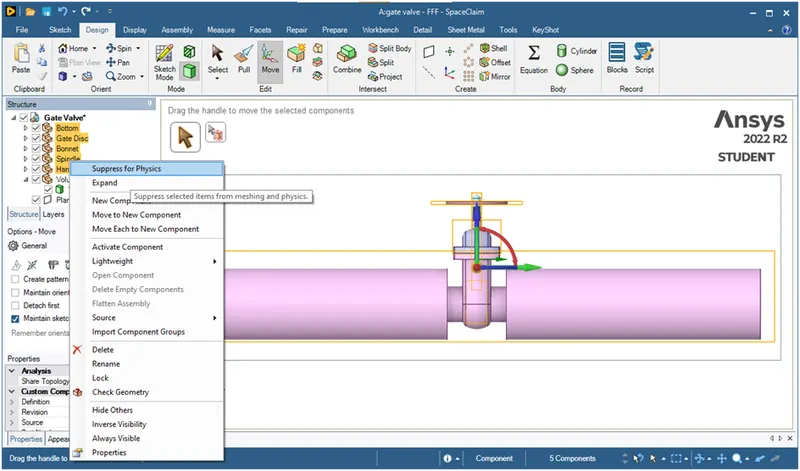
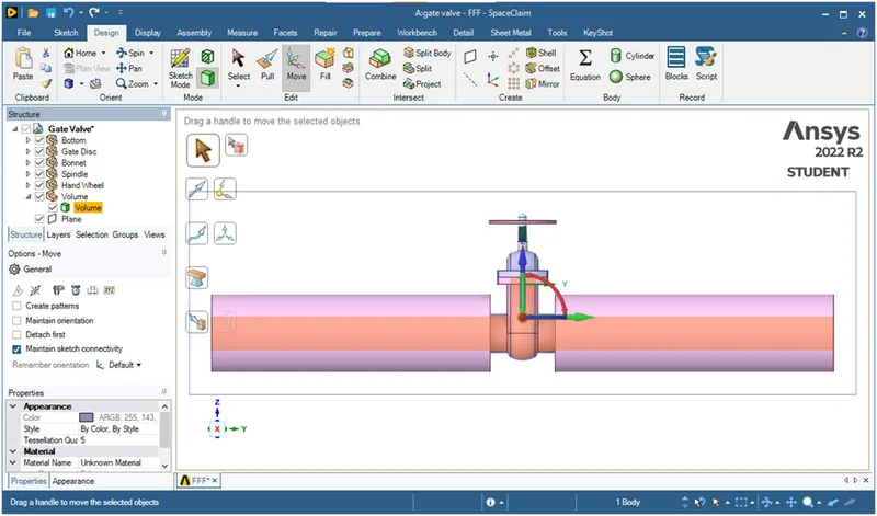
Now its done. We have successfully setup a parametric value as input as lift.

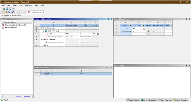
Lets goto meshing.

1.2. Meshing:

• Open meshing

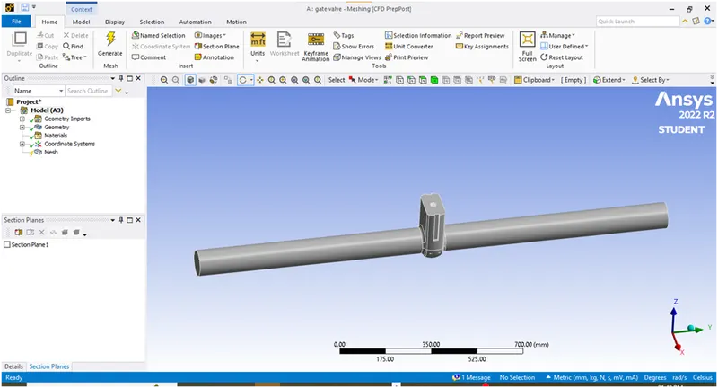
• Now right click on mesh and then click on generate mesh

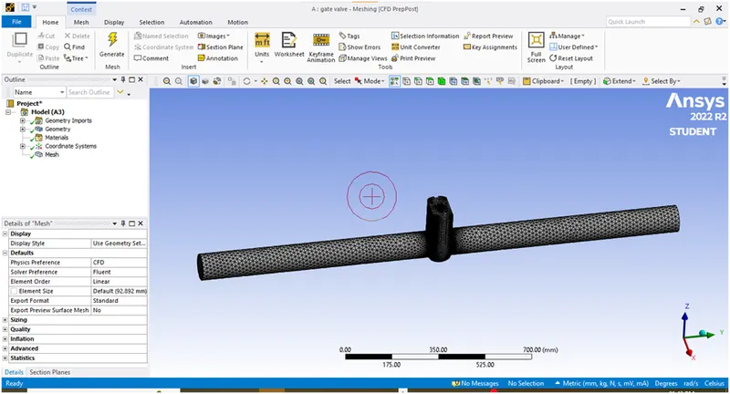
Let see sectional view.

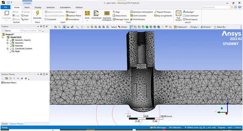
• Lets gives names to the faces s inlet, outlet and fluid volume as shown below.

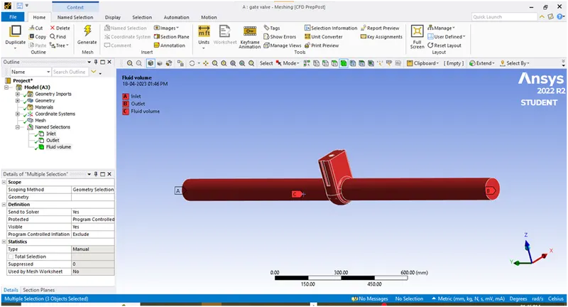
Now right click on mesh -> update mesh to transfer data to ansys fluent.

2. Post-processing methods:

2.1. Setup:

• Open setup with double precision and 4 processors

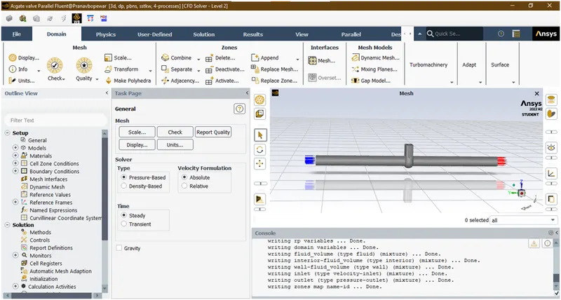
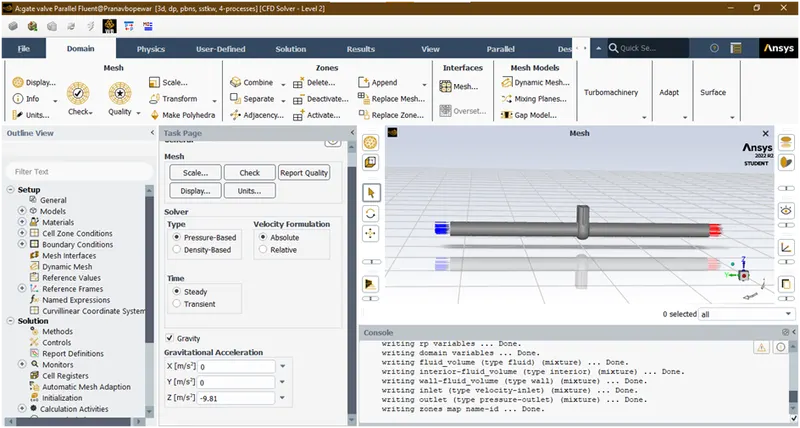
• Now enabele gravity in z-direction as -9.81 m/s².
• Used pressure based steady state solver.

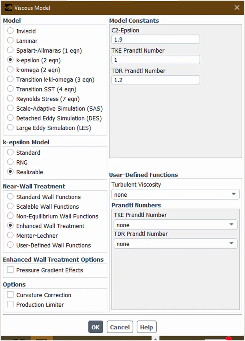
• Now goto models and enabled viscous-K-epsilon-realizable-enhanced wall treatment model to capture the near wall effects clearly.

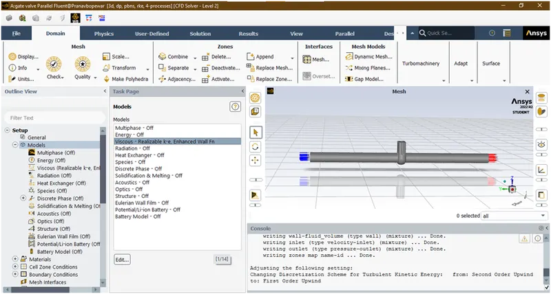
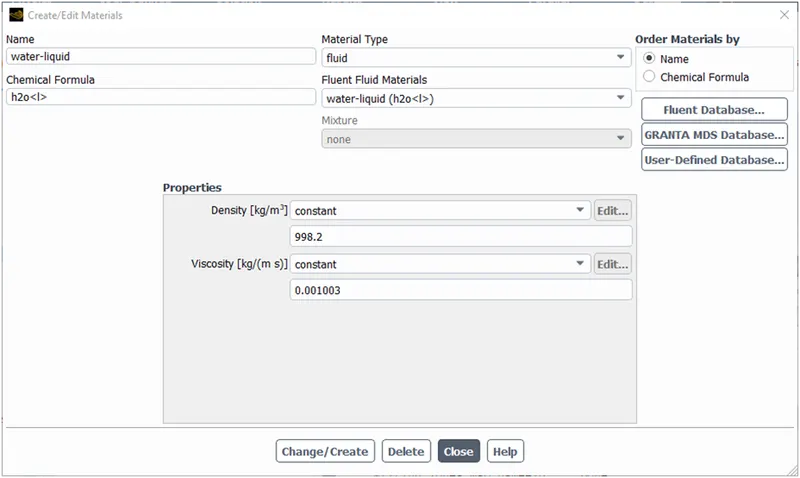
• Now goto materials and add water as a fluid

• Now goto cell-zone condition and apply fluid as a water

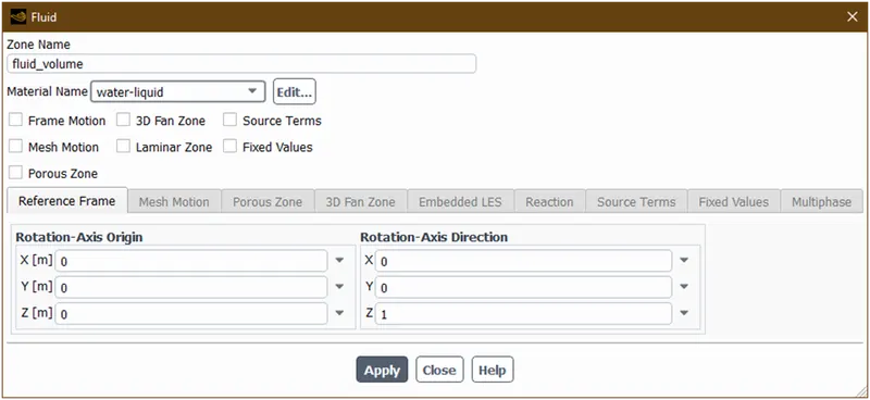
Then delete air from materials.

• Then goto boundary conditions

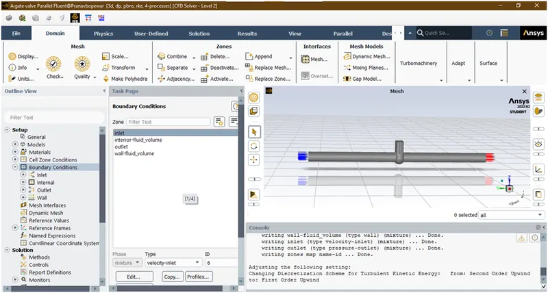
Now select the inlet and change type of inlet from velocity inlet to pressure inlet and give value as 10Pa.

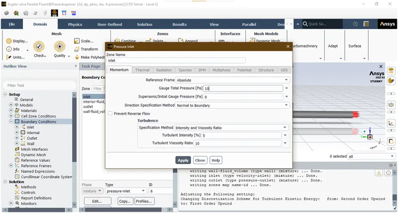
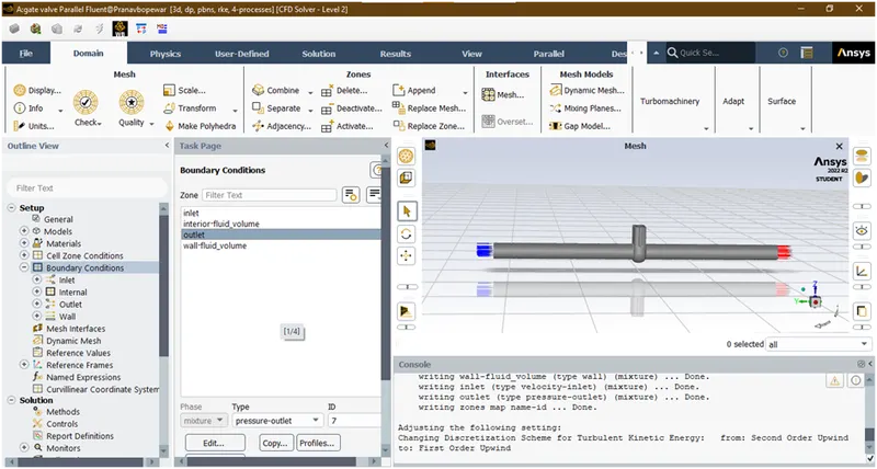
Lets check outlet as pressure outlet

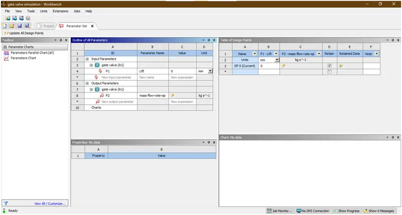
• Lets create report definition as mass flow rate at outlet and create as a output parameter as shown below.

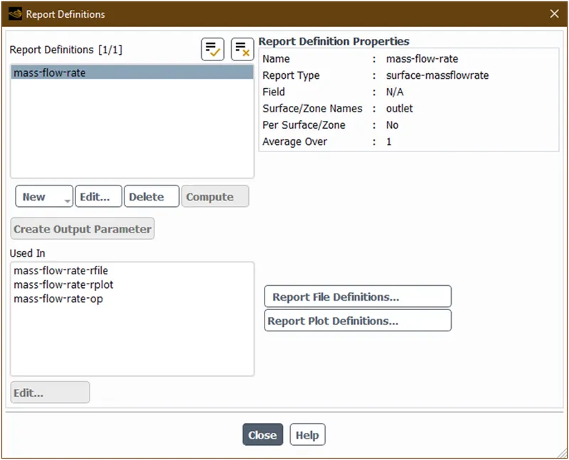
Let see is o/p parameter created or not

• Now initialize the solution
• Then run the calculation for 1000 iteration.
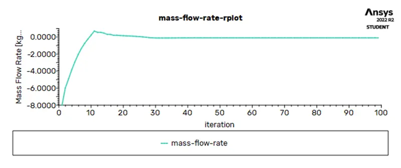
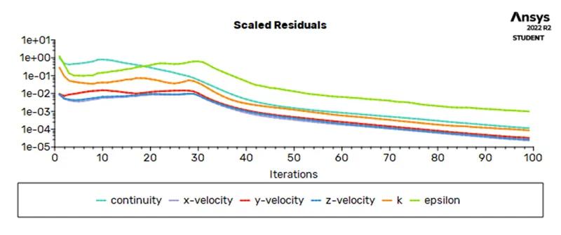
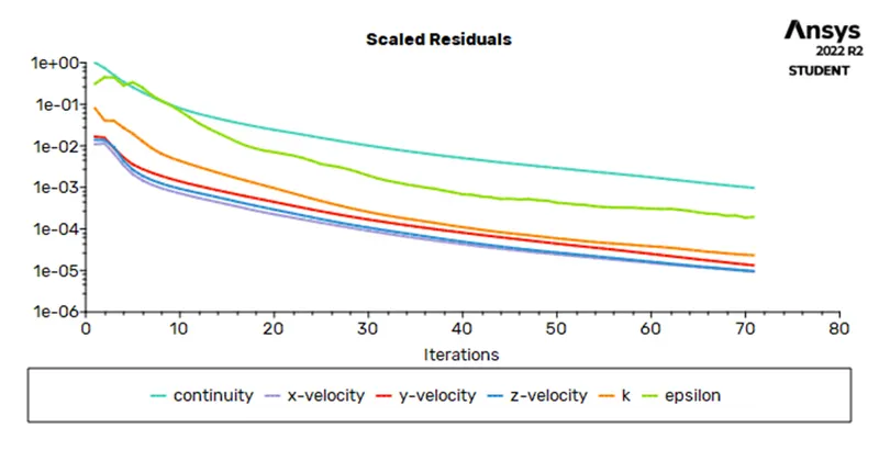
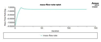
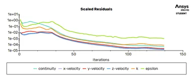
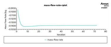
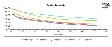
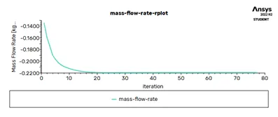
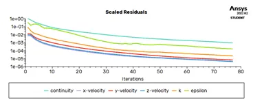
• After doing all just plot residual plot and mass flow rate plot

2.2. Results :

• Open cfd post
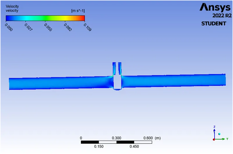
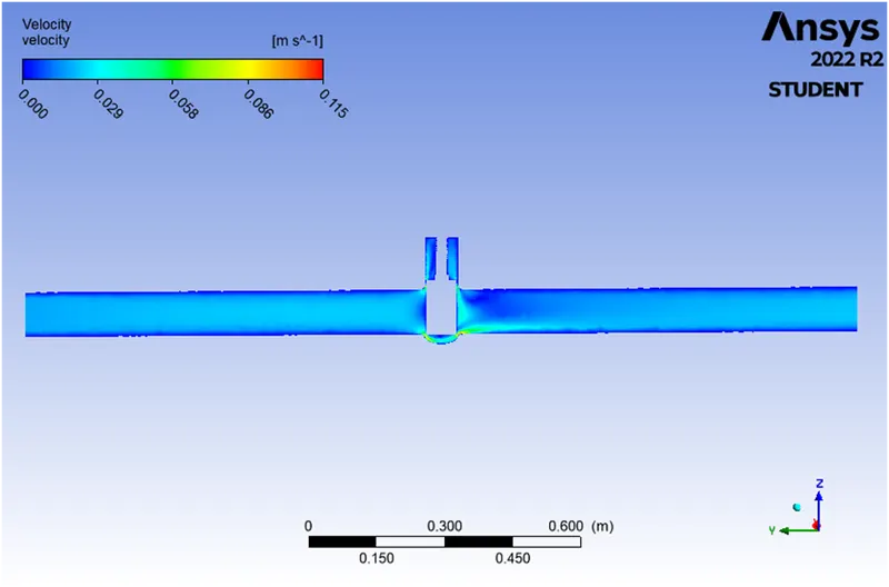
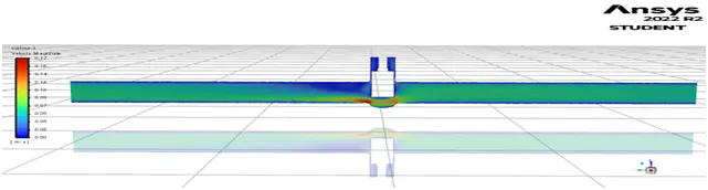
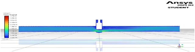
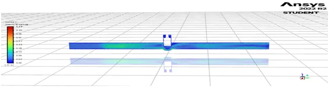
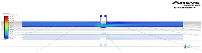
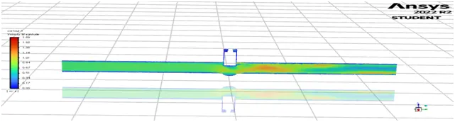
• Then plot velocity contour plot

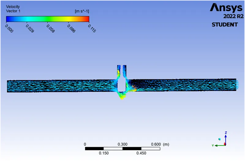
• Then plot velocity vector plot

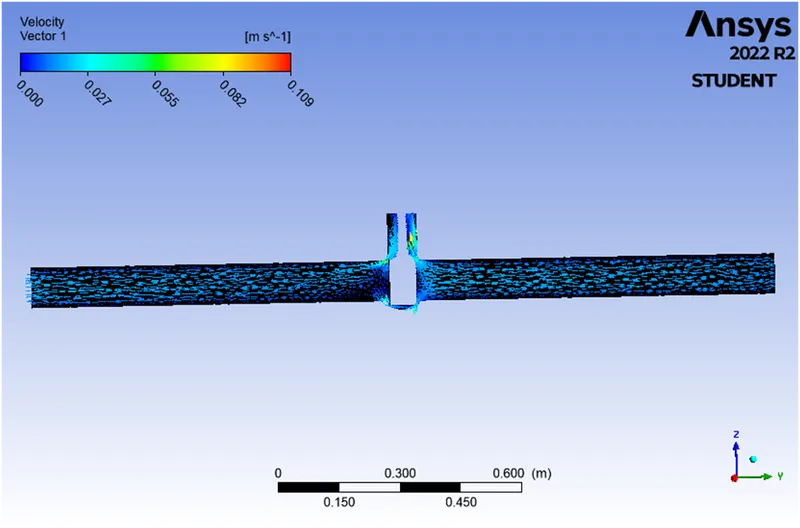
• After that open the parametric tab

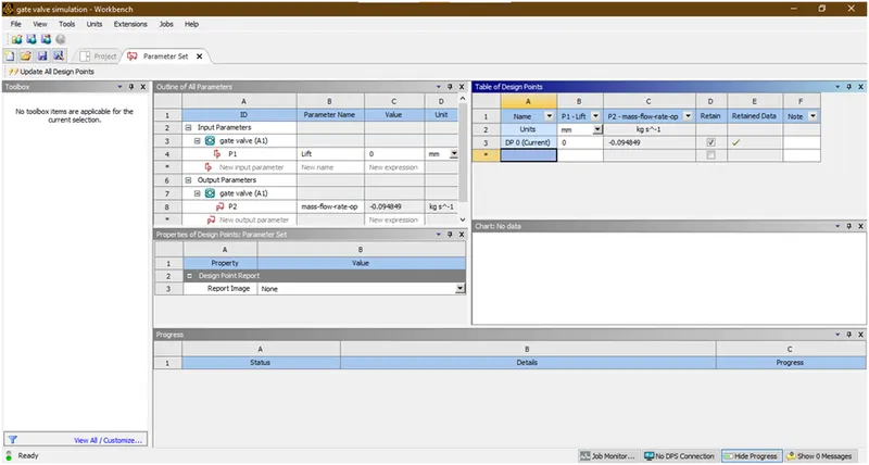
Give value=10 mm and click on radio button as shown below

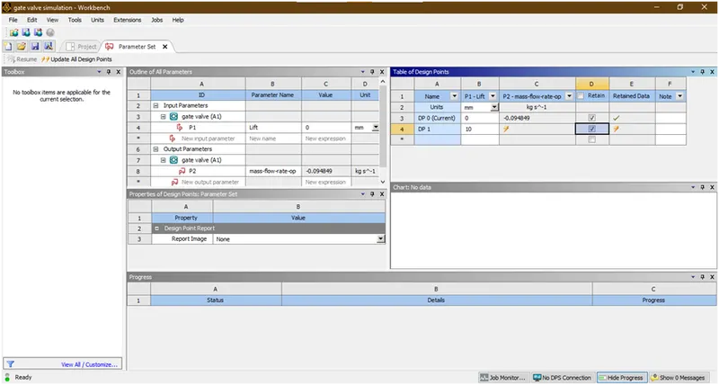
Now right click on dp1 -> update the design point

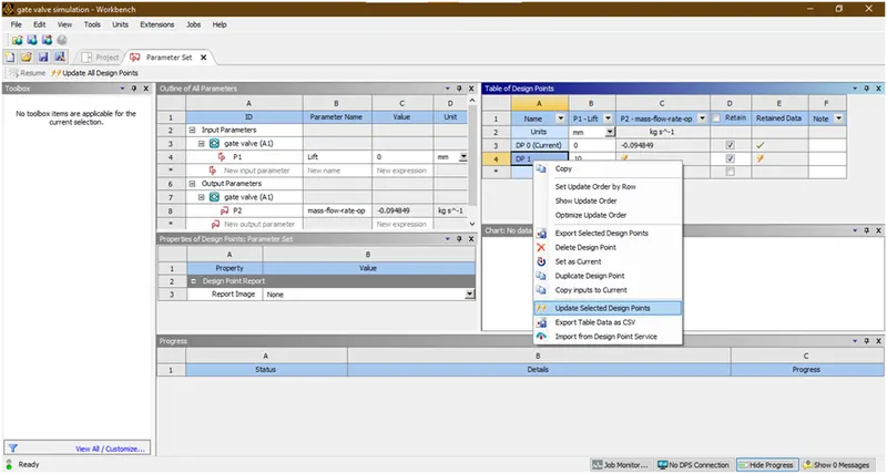
And wait until the solution generated

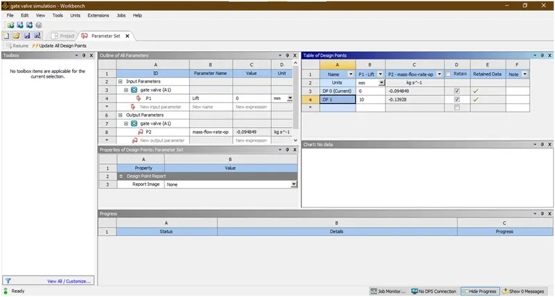
Now its done. To see plot just right click on DP1 and click on set as a current and then goto project scheme and plot a graphs

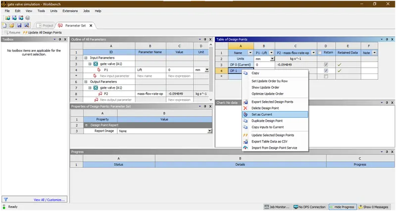
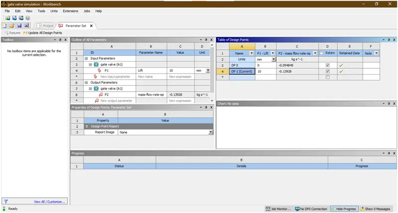
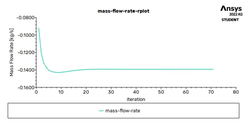
Now its done. Now further cases follow the same procedure as mentioned in this point.

Analytical calculations of flow factor and flow coe. :

Firstly calculate flow factor (K_v)

`Q=K_v sqrt((ΔP)/S)`

Here

S=1 for water

ΔP = P_i – P_o = 10-0 =10 Pa = 10 x 10^(-5) bar

`dotm`= ρQ

Where

ρ= density of fluid = 1000kg/m³

`dot m`= 0.09487 kg/s

Therefore, by putting these values we can get

Q= 0.09487 x 10^-3 m³/s = 0.09487 x 10^-3 x 3600 =0.3415 m³/hr

So flow factor(K_v)can be calculated as

`K_v=Qsqrt(S/(ΔP))=0.3415 ×sqrt(1/(10 xx10^(-5)))=`34.15

Now flow coe.(C_v) can be calculated as

K_v = 0.865 C_v

Therefore C_v = 34.15/0.865 = 39.48

Results :

• Parametric study

Case no.	Lift(mm)	Mass flow rate(kg/s)	Volume flow rate(m3/hr)	Flow factor (Kv)	Flow coe.(Cv)
1	0	-0.09569	-0.34448	-34.4484	-39.8247
2	10	-0.13879	-0.49964	-49.9644	-57.7623
3	20	-0.21909	-0.78872	-78.8724	-91.182
4	30	-0.33564	-1.2083	-120.83	-139.688
5	40	-0.43577	-1.56877	-156.877	-181.361
6	50	-0.49635	-1.78686	-178.686	-206.573
7	60	-0.48032	-1.72915	-172.915	-199.902
8	70	-0.59631	-2.14672	-214.672	-248.175
9	80	-5.0699	-18.2516	-1825.16	-2110.02

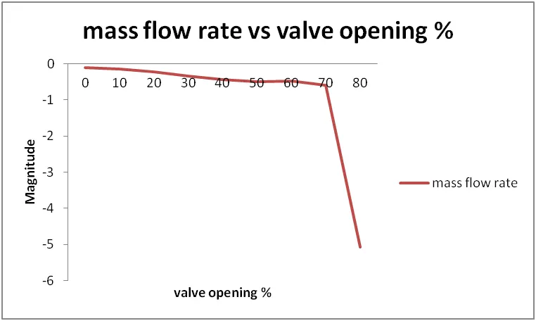
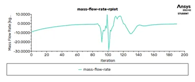
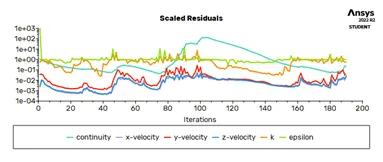
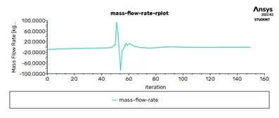
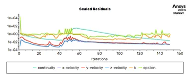
• Mass flow rate vs gate valve opening graph, flow factor vs gate valve opening, flow coe. Vs gate valve opening plots

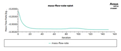
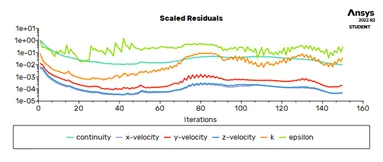
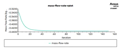
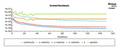
• Residual and mass flow rate plots

Case no.	Lift(mm)	Mass flow rate plots(kg/s)	Residual plots
1	0
2	10
3	20
4	30
5	40
6	50
7	60
8	70
9	80

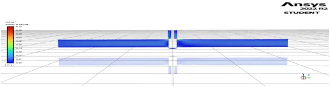
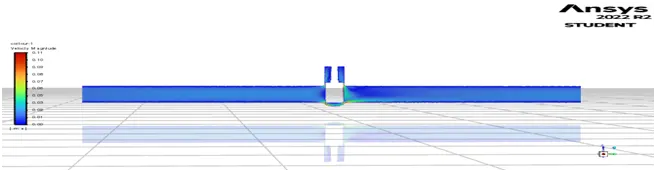
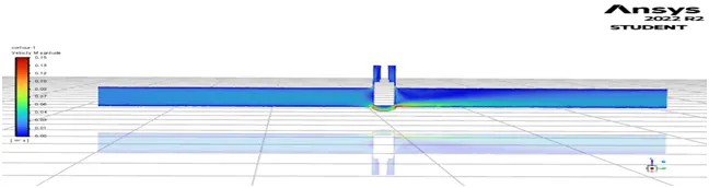
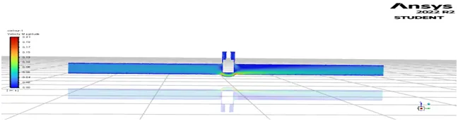
• Velocity contour plots and velocity vector plots

Case no.	Lift(mm)	Velocity contour plots
1	0
2	10
3	20
4	30
5	40
6	50
7	60
8	70
9	80

Conclusions:

1. From this challenge I have learn that, the parametric study is an easier method to find out the directly output value just once we have to setup. So it is a time reducing method i.e. optimizing method.
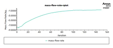
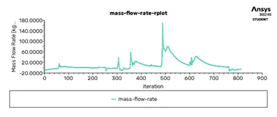
2. From this challenge and from tabular data and plots I can conclude that, as % of valve opening increases from 0 to 80%, the mass flow rate which will flow inside a pipe through valve is increased. Here in this table the values are comes in negative which simply denotes as its flow goes outside the volume.
3. Also flow rate, flow factor, and flow Coe. are depends upon the mass flow rate and properties of fluid and type of fluid. So as mass flow rate increases, these factors also increased.
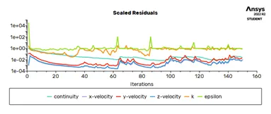
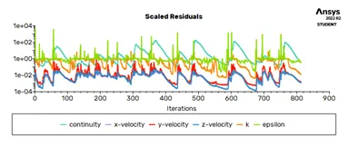
4. From mass flow rate plots wee can say that the solution gets converged within 200 iterations.
5. From velocity contour plots I can say that as mass flow rate increases the velocity of flow also increased at valve section.but these contour plots are drawn at instant so sometimes at that instant these variation in velocity not shown properly.