Week 9 - Parametric study on Gate valve.

Objective: To observe the sloshing effect of aa fluid in the gearbox.

Introduction:

Experiments performed to study the physics of certain phenomenon are costly and time-consuming. Numerical simulation is developed and used to reduce the time needed to study the nature and physics involved in the system of interest. This method indeed provides results very fast compared to experiments but they lack a bit in terms of accuracy. If the experiments take a month to produce results, simulation might take a day and give us results 90% accurate. In the fast-paced world, where developing various solutions require faster results, engineers make a delicate balance between the accuracy and time taken as necessary.

All fluid flows are governed by three equations -Continuity, momentum and energy equations. We need to solve these equations for the given conditions to understand the fluid behavior. Computers are incapable of solving these equations in their integral and differential forms. So, we can divide our geometry into many tiny elements (called mesh) and modify the governing equations into difference equations that can be solved by the computer. We apply these difference equations for all the elements in the geometry and generate an approximate solution. It is hence necessary to validate these results against the experimental data.

The number of difference equations, for a given problem varies with the nature of physics involved. We typically solve a finite number of equations at all the elements. These equations are grouped together, called a turbulence model. A lot of work has been put into developing and improving the turbulence models and the work still goes on today. Examples of turbulence models are S-A, k-epsilon, k-omega etc.

Theory:

Gate Valve:

A gate valve, also known as a sluice valve, is a valve that opens by lifting a barrier (gate) out of the path of the fluid. Gate valves require very little space along the pipe axis and hardly restrict the flow of fluid when the gate is fully opened. The gate faces can be parallel but are most commonly wedge-shaped.

Uses of gate valve:

Gate valves are used to shut off the flow of liquids rather than for flow regulation. When fully open, the typical gate valve has no obstruction in the flow path, resulting in very low flow resistance. The size of the open flow path generally varies in a nonlinear manner as the gate is moved. This means that the flow rate does not change evenly with stem travel. Depending on the construction, a partially open gate can vibrate from the fluid flow.

Modelling Approach:

The work flow in Ansys Fluent would follow four steps:

1. Geometry creation.
2. Mesh generation.
3. Pre-processing settings and simulation.
4. Extracting results.

Geometry creation:

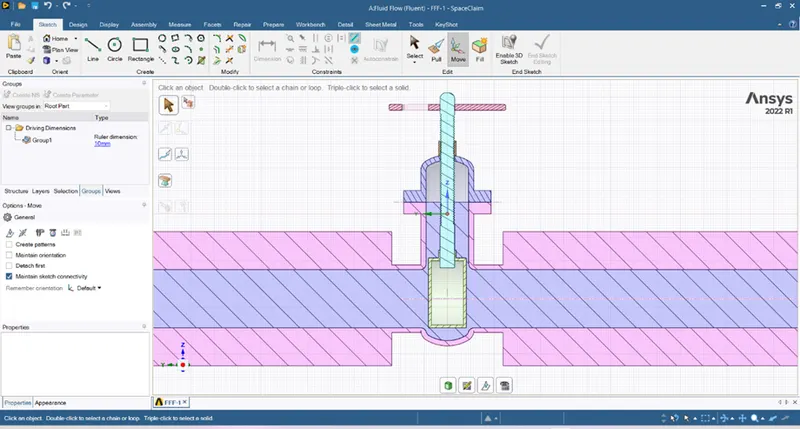
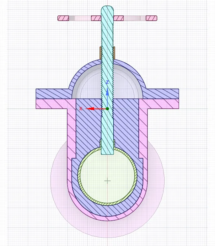
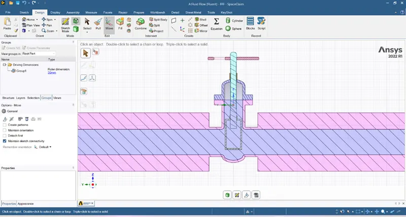
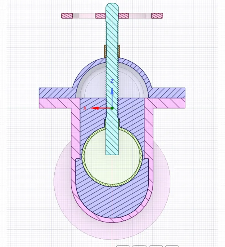
We drag and drop the Fluent module to create the standalone system. We open the geometry editing section- Space claim. We import the given geometry to Space claim. We use Move option to move the gate disc through 10mm and create a parameter in Groups section. We extend the inlet and outlet by 800mm to create the fluid volume.

We need to extract the fluid volume using Prepare -> Volume Extract. We create co-ordinate planes at origin. We now cut the fluid volume in half across XY plane to visualize the lift in gate disc for 10mm and 30mm as shown.

Mesh generation:

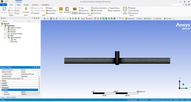
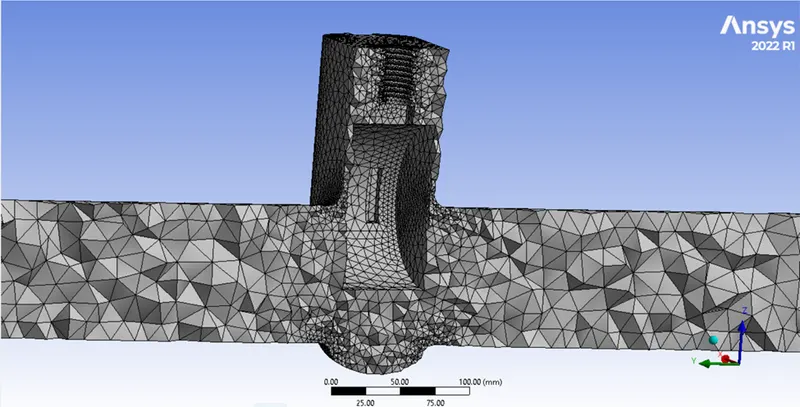
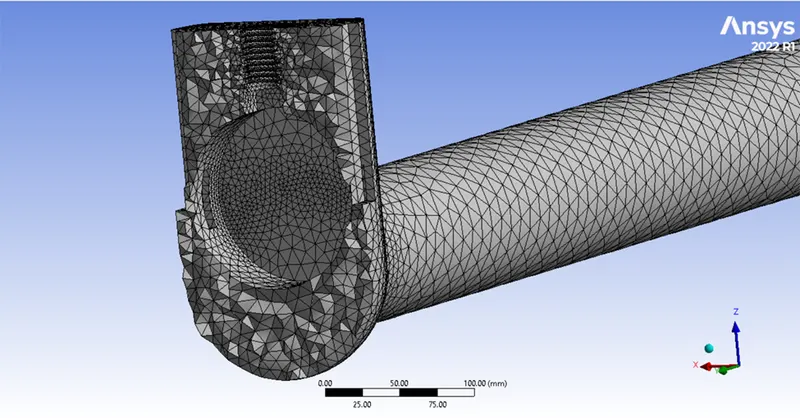
We generate the mesh with the default value of mesh length as 92 mm. We assign appropriate named selections to make it easier to work in the simulation section later. Here, we assigned the names for inlet and outlet. We close the window and the changes are updated in the system.

Pre-processing settings and Simulation:

We would proceed to Setup the conditions of the model. The process flow would be as follows:

1. Check the mesh in the solver.
2. Choose the turbulence model.
3. Specify boundary conditions and cell zone conditions.
4. Create necessary surface plots that we need to investigate.
5. We initialize and run the simulation for given number of iterations

Extracting results:

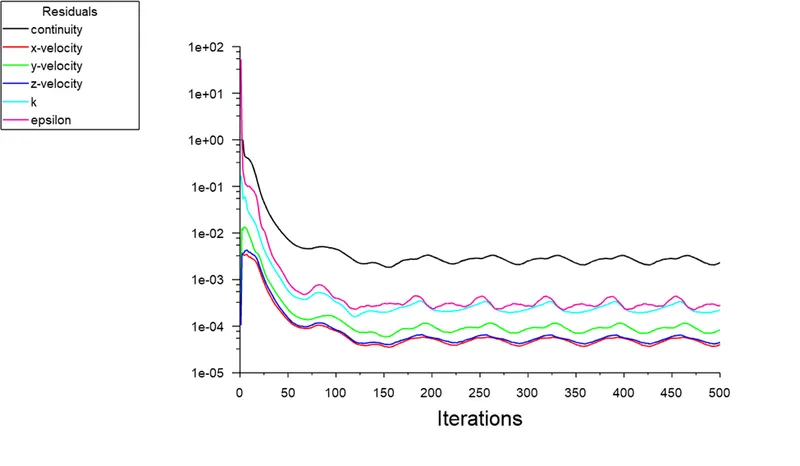
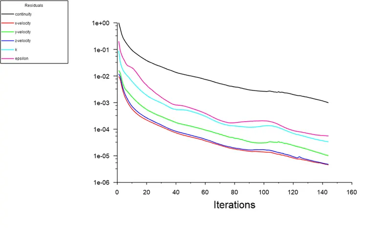
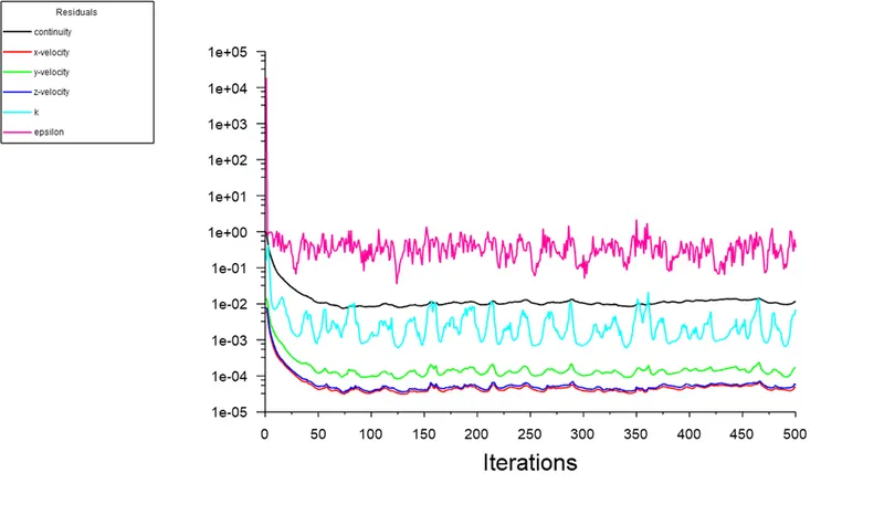
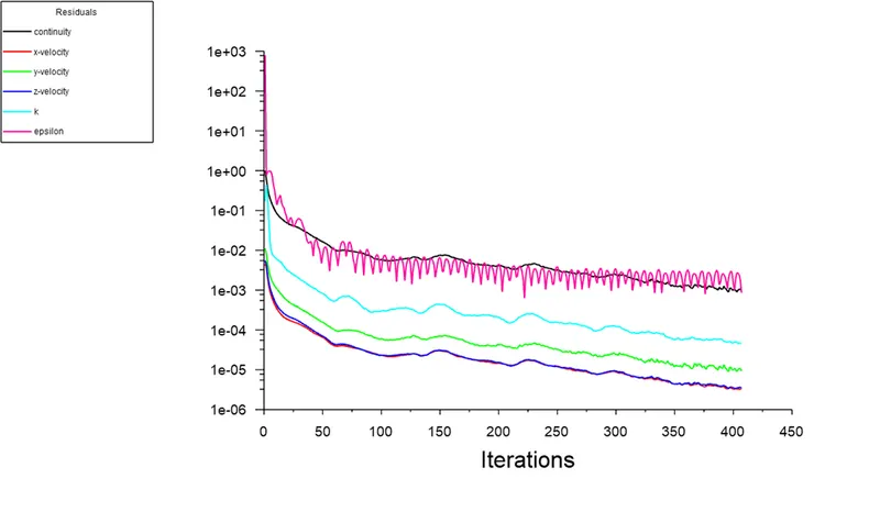
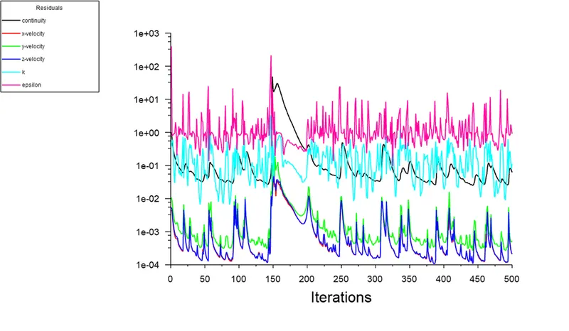
We open the results section where we can use various visualizing tools like transparency and colouring the created surfaces with the instantaneous variables like temperature, velocity and obtain contours, charts, plots and animations. We need to run the simulation until the residual values are either reach the convergence criteria or display a periodic pattern.

Settings used for current simulation:

We used Pressure-based solver, absolute velocity formulation, steady state simulation and enable gravity.

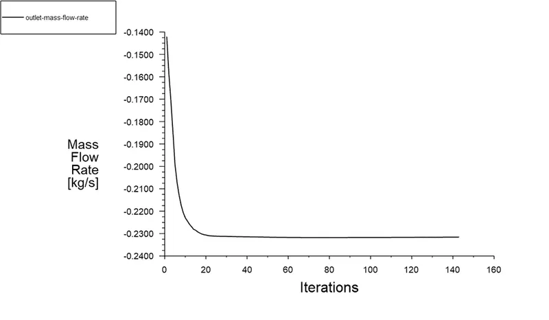
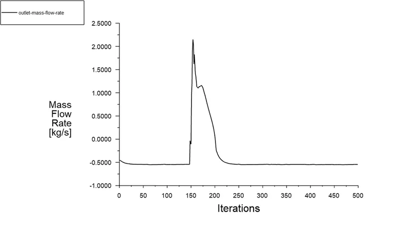
We used RNG k-epsilon turbulence model with swirl dominated flow. We use water as working media. We use pressure inlet and input gauge pressure as 10Pa. We create an output parameter for mass flow rate at outlet and run the simulation.

Case 1: Lift-10mm:

Scaled Residuals:

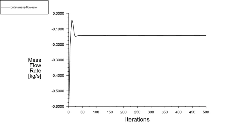
Outlet mass flow rate:

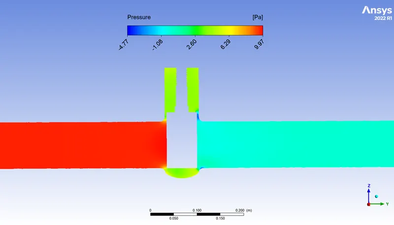
Pressure contour:

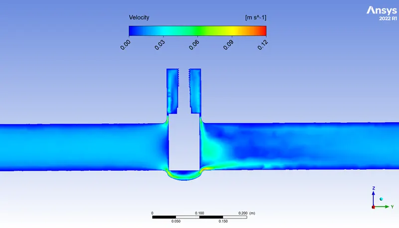
Velocity contour:

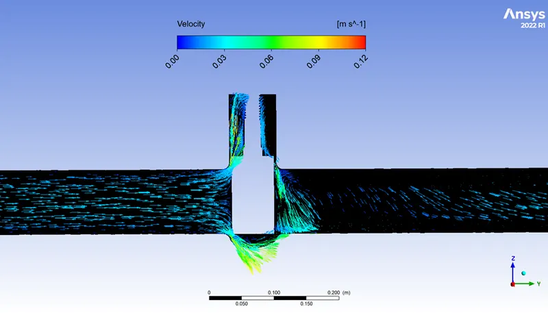
Velocity vector:

Parametric study:

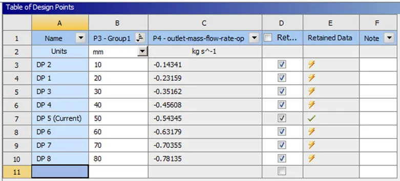
Once we are done with 10mm lift simulation, we can go to parameters option in workbench. We can input the next value of lift and use Update to selected design points. Ansys would modify the geometry, create mesh and run simulation based on the already present boundary conditions. Once the simulation is complete, we get the mass flow rate at outlet in the parameter window. We can access the plots required by selecting Set as current option. The final data with all lift cases can be seen.

Case 2: Lift-20mm:

Scaled Residuals:

Outlet mass flow rate:

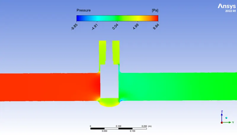
Pressure contour:

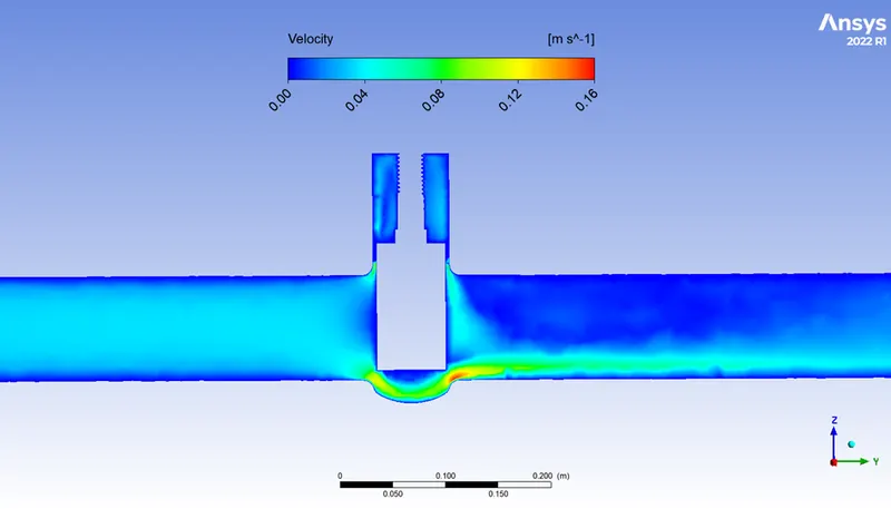
Velocity contour:

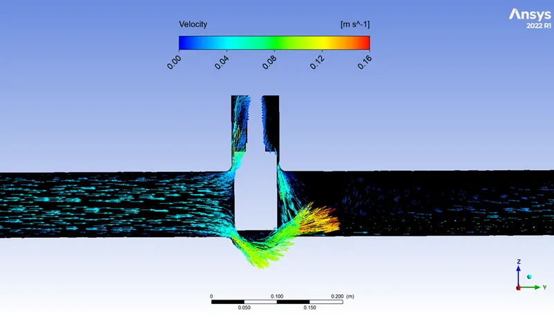
Velocity vector:

Case 3: Lift-30mm:

Scaled Residuals:

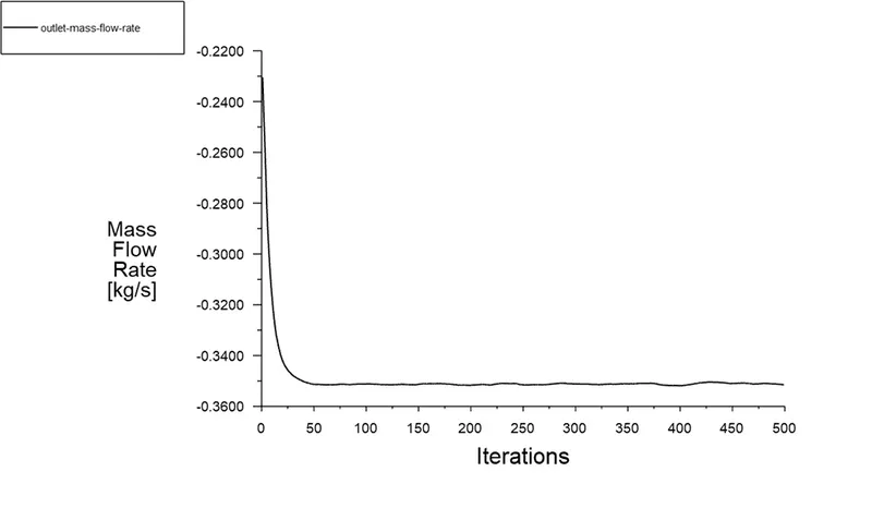
Outlet mass flow rate:

Pressure contour:

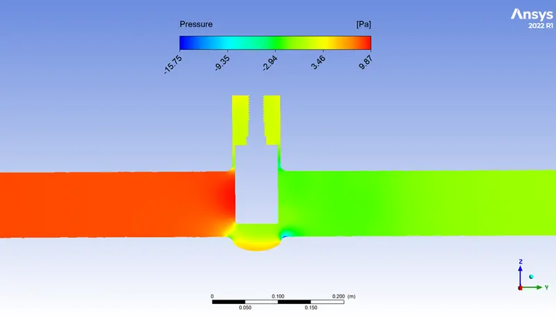
Velocity contour:

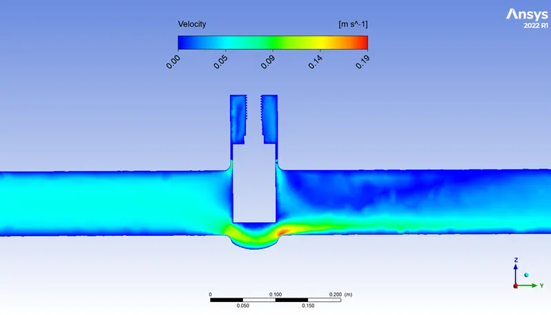
Velocity vector:

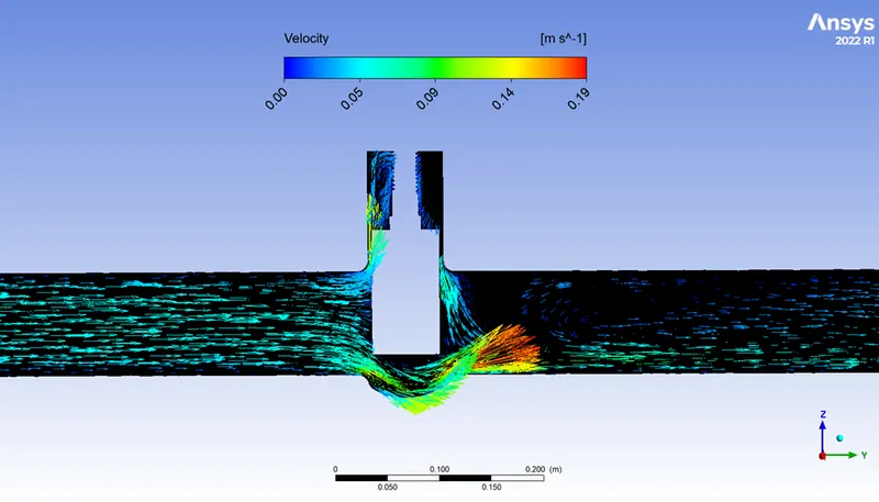
Case 4: Lift-40mm:

Scaled Residuals:

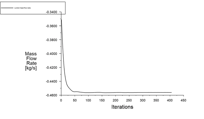
Outlet mass flow rate:

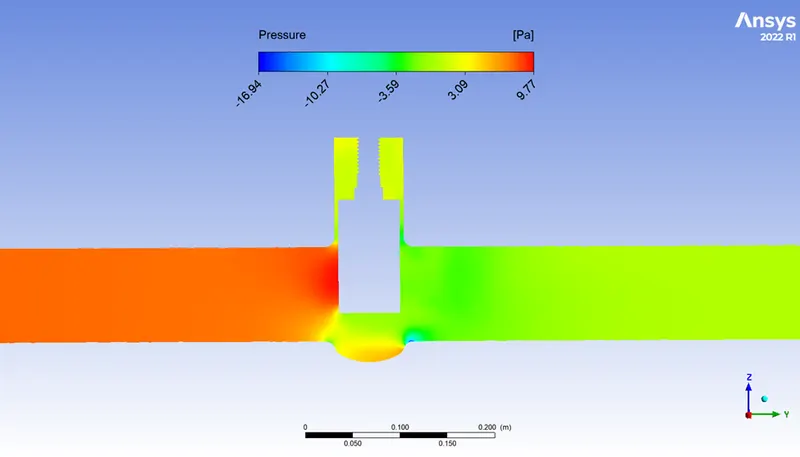
Pressure contour:

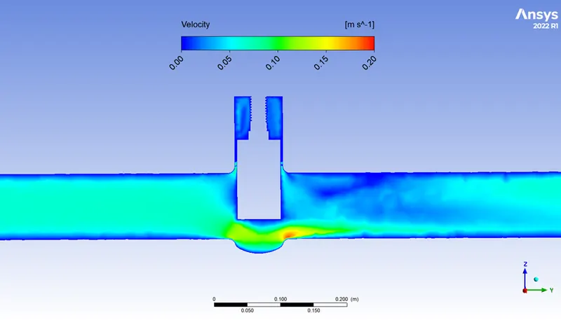
Velocity contour:

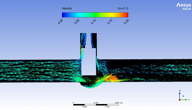
Velocity vector:

Case 5: Lift-50mm:

Scaled Residuals:

Outlet mass flow rate:

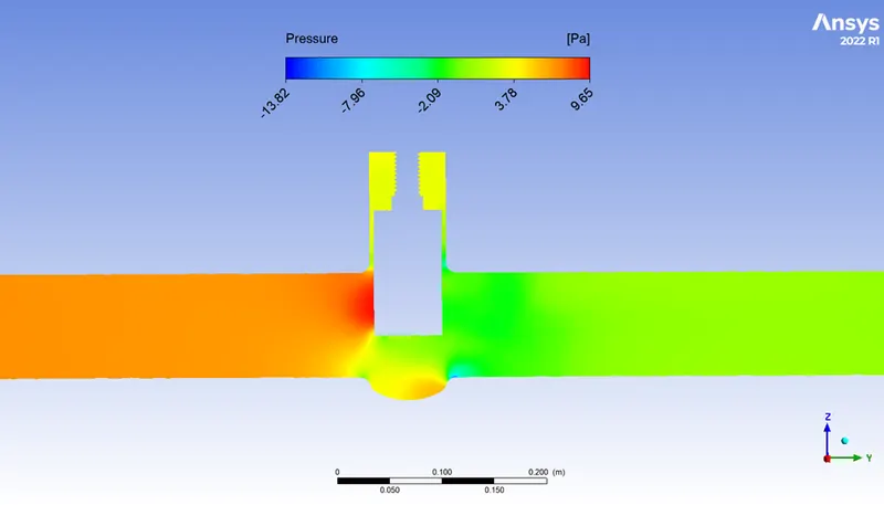
Pressure contour:

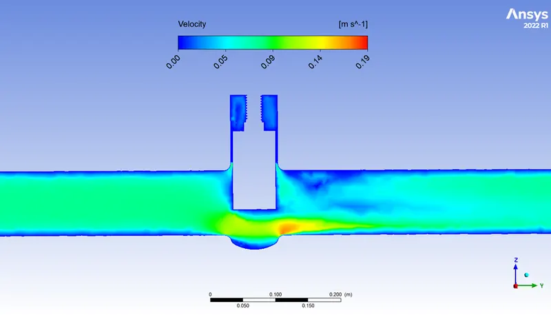
Velocity contour:

Velocity vector:

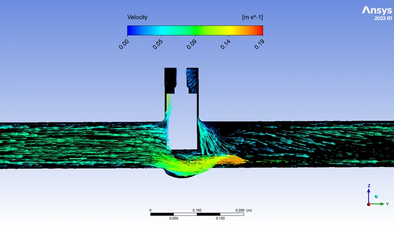
Case 6: Lift-60mm:

Scaled Residuals:

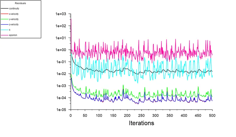
Outlet mass flow rate:

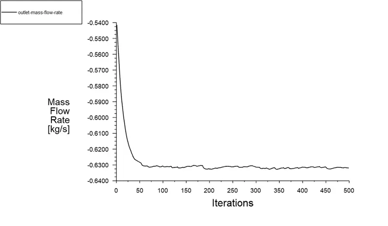
Pressure contour:

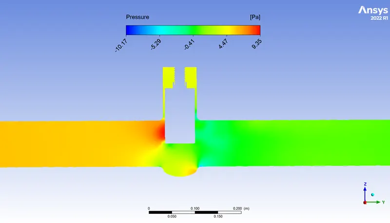
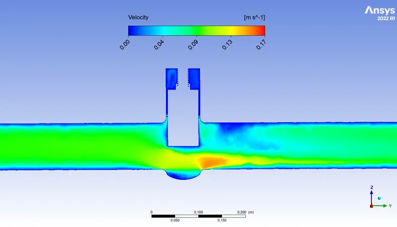
Velocity contour:

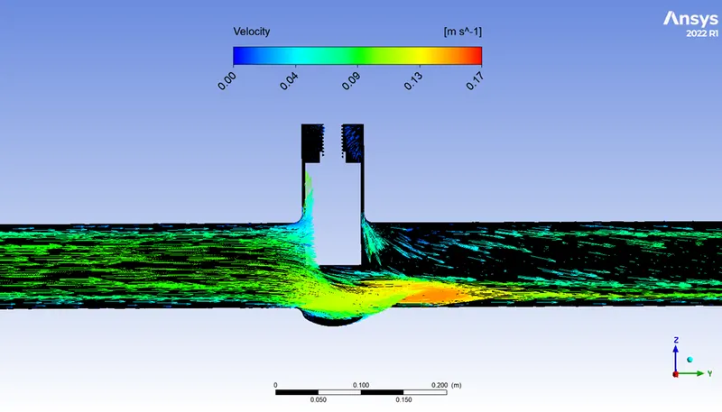
Velocity vector:

Case 7: Lift-70mm:

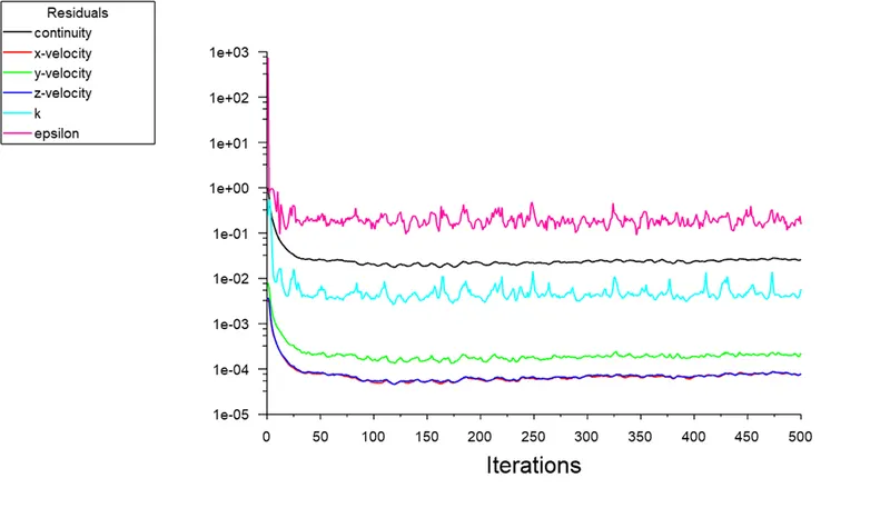
Scaled Residuals:

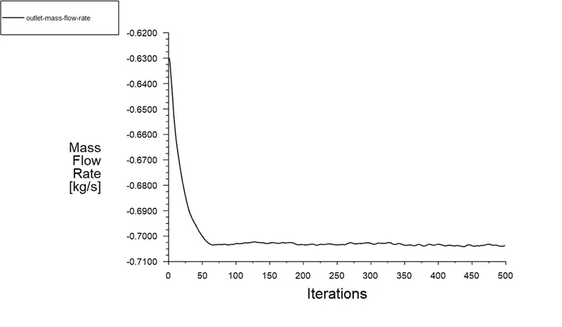
Outlet mass flow rate:

Pressure contour:

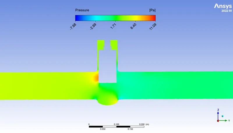
Velocity contour:

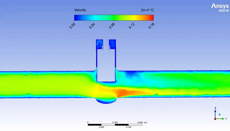
Velocity vector:

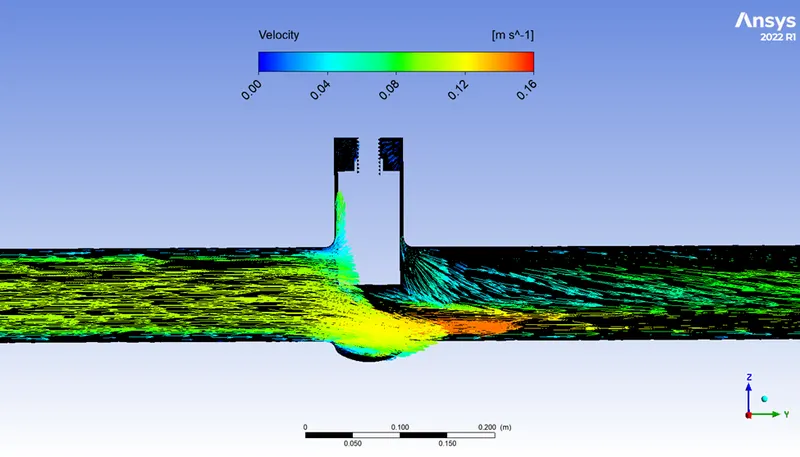
Case 8: Lift-80mm:

Scaled Residuals:

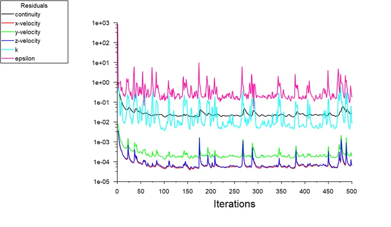
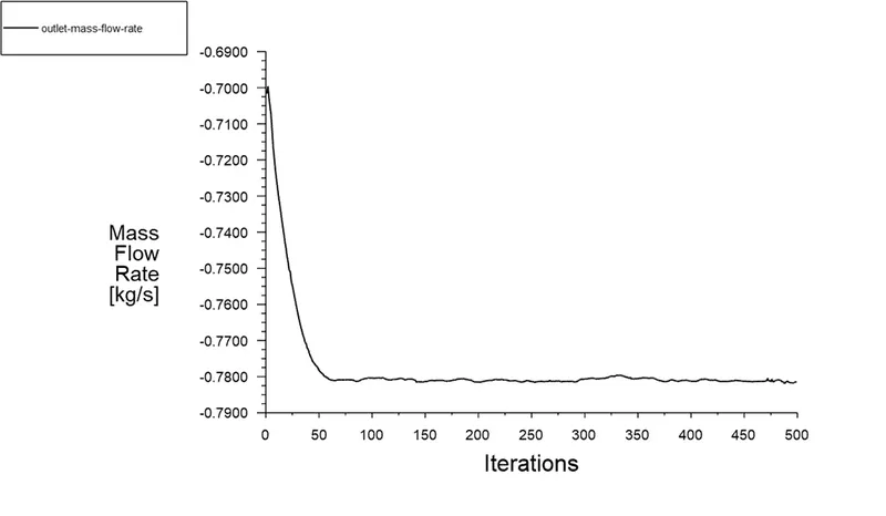
Outlet mass flow rate:

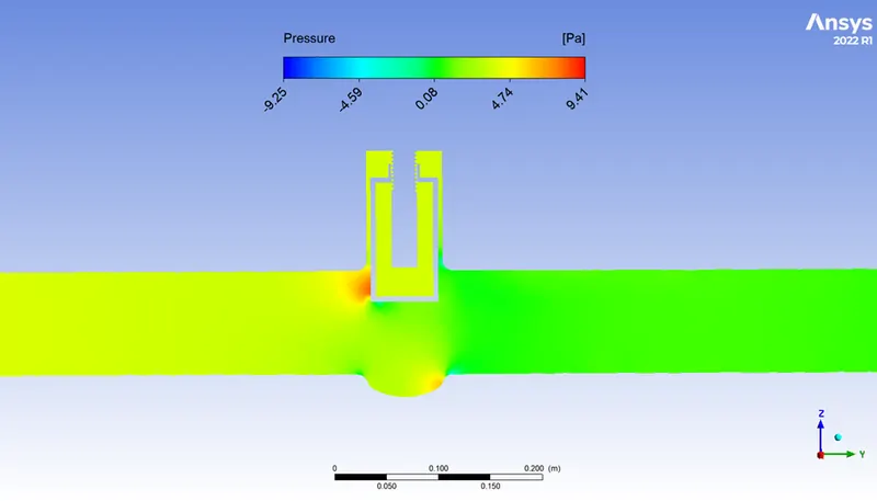
Pressure contour:

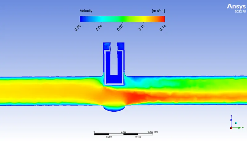
Velocity contour:

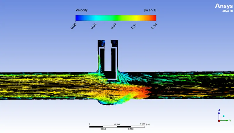
Velocity vector:

Analytical solution:

The data for 10mm lift are:

Mass flow rate Q = 0.14341 kg/s, Pressure drop P = 10 Pa, specific gravity = 1

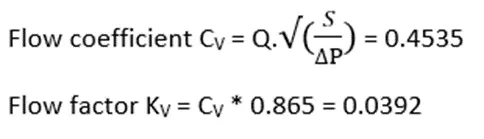
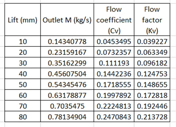
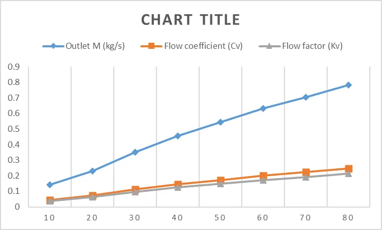
Similarly, we can calculate values for other cases. The data is tabulated and plotted.

Conclusion:

It can be inferred that with increase in the lift of gate disc, the values of mass flow rate, flow coefficient and low factor increases. Parametric study helps us to simulate the results for a geometry with a change in parameter easily. We can save time needed for analysis using this feature.