Week 3 - Solving second order ODEs

Objective: To calculate the motion of the pendulum using differential equation defining simple harmonic motion and animate the result.

Theory: The motion of a pendulum depends on Newton’s second law. The instantaneous position of the bob at given angle θ to the vertical is defined by the following equation.

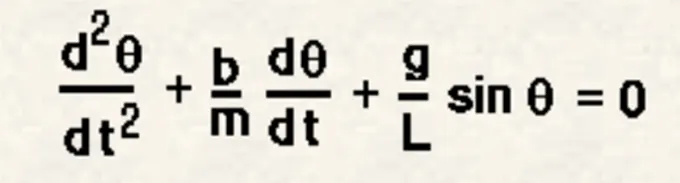
Where θ = angle made by pendulum with the vertical

b = damping coefficient

m= mass of the bob

g = acceleration due to gravity

L = length of the pendulum

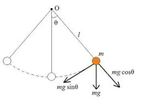
The following input parameters are given to solve the differential equation.

b = 0.05; m = 1 kg; L = 1 m; g = 9.81 m/ .

Initial condition of pendulum – At time t = 0, θ = 0, = 3 rad/s .

Code:

The second order differential equation is broken down into two first order differential equations. We have written the function ode_func to define the two first order differential equations.

The inbuilt ode45 solver is used to solve differential equations by passing ode_func function and initial parameters in ode45 syntax as mentioned in the code.

Function code:

% ode_func function definition
 
function [dtheta_dt] = ode_func(t,theta,b,g,l,m)
 
theta1 = theta(1);
theta2 = theta(2);
dtheta1_dt = theta2;
dtheta2_dt = -(b/m)*theta2 - (g/l)*sin(theta1);
dtheta_dt = [dtheta1_dt; dtheta2_dt];
 
end

------------------------------------------------------

Main code:

%solving second order ODE
 
clear all
close all
clc
 
b = 0.05;
g = 9.81;
l = 1;
m = 0.1;
 
%initial condition
theta_0 = [0;3];
 
%time points
t_span = linspace(0,20,500);
 
%solve ODE
 
[t, results] = ode45(@(t,theta) ode_func (t, theta, b, g, l, m), t_span, theta_0);
 
subplot(2,1,1)
plot(t, results(:,1));
xlabel('time in s');
ylabel('angular displacement');
hold on
subplot(2,1,2)
plot(t, results(:,2));
ylabel('angular velocity')
xlabel('time in s')
grid on;
 
%Animating the plot
 
x0 = 0;
y0 = 0;
 
ct=1;
for i= 1:length(t_span)
    x1 = l*sin(results(i,1));
    y1 = -l*cos(results(i,1));
    
    figure(2)
    plot([-1 1],[0 0],'linewidth',10,'color','b');
    axis([-2 2 -2 2]);
    line([x0 x1],[y0 y1],'linewidth',5,'color','g');
    hold on;
    plot(x1,y1,'O','markersize',20,'markerfacecolor','r');
    title('Damping of pendulum animation');
    legend('Wall','length of pendulum','bob of pendulum');
    grid on;
    hold off;
    text(-1,1,sprintf('Angular displacement = %f',results(i,1)));
    text(-1,0.8,sprintf('Angular velocity = %f',results(i,2)));
     M(ct) = getframe(gcf);
     ct = ct+1;  
end
 
movie(M);
videofile = VideoWriter('pendulum animation.avi','Uncompressed AVI');
open(videofile)
writeVideo(videofile,M)
close(videofile)

Result:

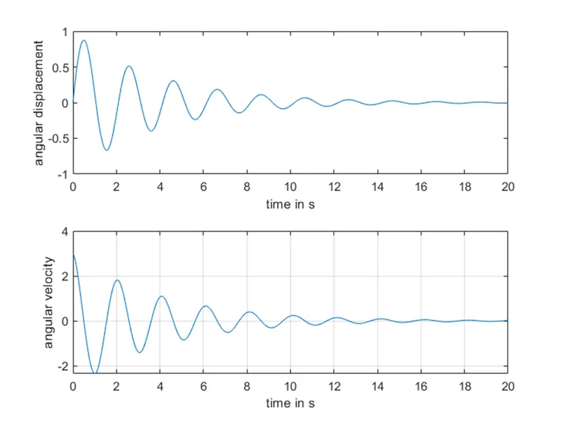
The motion of the pendulum is animated using the given parameters. The video is available in the following link.

https://www.youtube.com/watch?v=gUK2DvJWVD8&list=PLM7Ccs99CHRB-lZFwRFwgAbrnaYDiiaeP&index=2

The change in angular displacement and angular velocity w.r.t. time is plotted.

Conclusion:

The motion of pendulum following simple harmonic motion is calculated for the given parameters using the given differential equation and is animated.