Week 9 - Parametric study on Gate valve.

Parametric study on a Gate Valve :

Aim : To analyze the mass flow rate through the outlet of a Gate valve for different valve openings by parameterizing the valve opening.

Objectives : 1. To parameterize the quantity "valve opening".

2. Using the appropriate boundary conditions and turbulence model.

3. Analyze the mass flow rate at the outlet.

Part-I :

Theory:

A Gate Valve :

A gate valve, also known as a sluice valve, is a valve that opens by lifting a barrier (gate) out of the path of the fluid. Gate valves require very little space along the pipe axis and hardly restrict the flow of fluid when the gate is fully opened. The gate faces can be parallel but are most commonly wedge-shaped (in order to be able to apply pressure on the sealing surface).

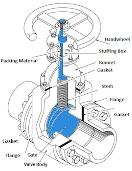
Components of a Gate Valve :

Working of a Gate Valve :

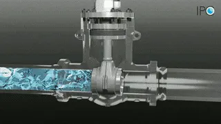
Common gate valves are actuated by a threaded stem that connects the actuator (e.g. handwheel or motor) to the gate. They are characterised as having either a rising or a nonrising stem, depending on which end of the stem is threaded. Rising stems are fixed to the gate and rise and lower together as the valve is operated, providing a visual indication of valve position. The actuator is attached to a nut that is rotated around the threaded stem to move it.

Uses of a Gate valve :

Gate valves are used to shut off the flow of liquids rather than for flow regulation. Gate valves are mostly used with larger pipe diameters (from 2" to the largest pipelines) since they are less complex to construct than other types of valves in large sizes.

Gate valves without an extra sealing ring on the gate or the seat are used in applications where minor leaking of the valve is not an issue, such as heating circuits or sewer pipes.

Flow coefficient (`C_v`):

The flow coefficient of a device is a relative measure of its efficiency at allowing fluid flow. It describes the relationship between the pressure drop across an orifice valve or other assembly and the corresponding flow rate.

Mathematically the flow coefficient `C_v` (or flow-capacity rating of valve) can be expressed as:

`C_v = Q*sqrt((SG)/(DeltaP))`

where, Q is the flow rate expressed in US Gallons per minute.

SG is the specific gravity of the medium flowing through the valve (For water, SG = 1)

`Delta P`is the pressure drop across the valve (expressed in PSI).

In more practical terms, the flow coefficient C_v is the volume (in US gallons) of water at 60 °F that will flow per minute through a valve with a pressure drop of 1 psi across the valve.

The use of the flow coefficient offers a standard method of comparing valve capacities and sizing valves for specific applications that is widely accepted by industry.

Flow factor (`K_v`) :

The metric equivalent of the flow coefficient is the flow factor which is calculated using the metric units.

Mathematically,

`K_v = Q*sqrt((SG)/(DeltaP))`

Here,

`K_v` is the flow factor expressed in `m^3/(hr)`.

SG is the specific gravity of the medium flowing through the valve (For water, SG = 1)

`Delta P`is the pressure drop across the valve (expressed in bar).

`K_v` can be calculated from `C_v` using the expression :

`K_v = 0.865*C_v`.

It is also to be noted that The k_v factor of a valve indicates "The water flow in m³/h, at a pressure drop across the valve of 1 kgf /cm² when the valve is completely open. The complete definition also says that the flow medium must have a specific gravity of 1000 kg/m³ and a kinematic viscosity of 10⁻⁶ m²/s. e.g. water.

------- - - - -.. . ----- -- -- - -- - - ------- -------- ------------------ ----- - --------- --- --- - - --- --- ------ -- ---- --- -------------

Modelling the Gate Valve :

Step.I :

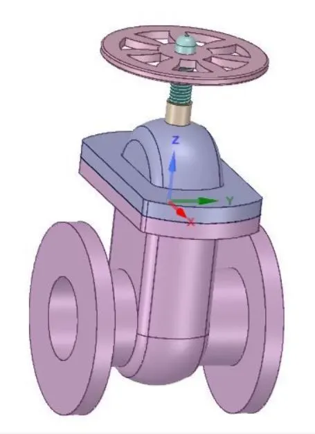
The 3D CAD geometry file is imported into the SpaceClaim component of the Fluid flow(FLUENT) analysis system.

Step.II : Extracting the fluid volume

In the "Prepare" tab of the SpaceClaim, click on the Volume extract tool and then click on the edge selection tool.

Click on the edge that represents the circumference of the inlet, outlet and the bonnet. Then click on the tick mark so that the fluid volume gets extracted.

Step.III : Creating the parameter P for the "gate displacement"

Hide all the components except the Gate disc. Click on the "Move" option available in the design toolbar. Use the component select feature and move the gate disc in the + Z-direction by 10 mm. Just after doing this, click on the "P" symbol that stands for the Parameter.

When this step is executed correctly, the message "New group is created" is displayed in the message pane.

Step.IV : Updatation of the Fluid volume

Now hide all the components except the "fluid volume". Expand the component and right click on it. Now click on the option "Update the volume by the context".

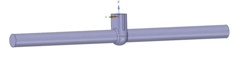
Step.V : Supress all the components for physics except the fluid volume. After this step, using the "Pull" tool extend the inlet and outlet surfaces of the geometry by 800 mm or any length greater that this. This step is to performed to so as to make the geometry long enough to visualize the fully developed flow during the entry and after passing through the valve.

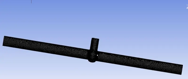
The final geometry looks as follows :

Meshing :

Once the Mesher tool is launched and the geometry is loaded successfully loaded, name the inlet and outlet using the Named selection feature.

Click on the generate mesh button and a baseline mesh is generated. To setup a fine mesh, change the element size to 6mm and click on "Update Mesh"

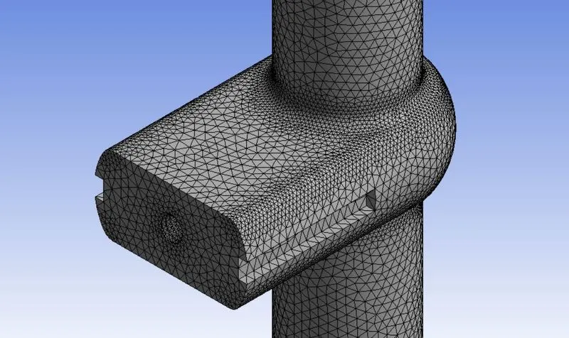
A finer mesh with the node count of 87339 and element count of 414055 is generated.

A close up of the mesh at the valve location :

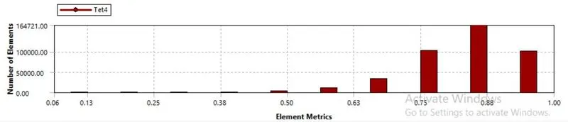
Mesh metrics :

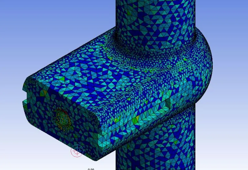
a. Element quality

b. Element size :

Setting up the case in ANSYS FLUENT :

Launch the ANSYS FLENT setup component from the analysis system. When the mesh is loaded into the FLUENT, check for the Mesh using the "Check Mesh" tool.

Any recommendations made by the FLUENT such as improving the mesh quality or reconstruction of the model can be made then and there.

The following are the physics that are defined so as the setup the case :

1. Gravity : -9.81 m/s^2 in the +Z-direction.

2. Steady state with K-epsilon realizible vicous model with scalable wall functions.

3. Water (H2O-Liquid) as the medium that flows through the fluid volume.]

Specification of the Turbulence model :

After seeting up a case and initializing with the values at the inlet it is found that the flow velocity is 0.141 m/s.

The results can be used for the calculation of the reynolds number which is `Re = (rho * V * D)/(mu)`

Here, `rho`is the density of water which has the value of 999.84 at 15 deg. centigrade.

V = fluid velocity for 10 mm gate displacement (In our case V= 0.141 m/s)

D = characteristic length, which is the pipe diameter (In our case D = 0.05 m)

`mu` = absolute/ dynamic viscosity of H2O at 15 deg. centigrade = 1.31 mPa.s

Hence `Re = (999.84 * 0.141*0.05)/(1.131*10^-3)`

= 6336.76

This value of Re is well above the value of a critical reynolds number for a pipe flow. Hence we use the K-epsioln turbulence model with scalable wall functions.

Setting up the boundary conditions :

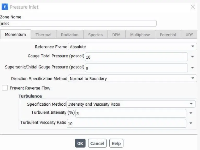
1. Inlet boundary condition :

Change the type of the inlet to "Pressure inlet". This can be done by right clicking on the inlet and floowing the step shown as follows:

Inlet > type > Pressure inlet.

In the text box where the Inlet gauge pressure has to be input, type in the value of 10 Pa.

2. Oulet boundary condition :

Pressure outlet with the default parameters.

3. Wall boundary condition :

Walls with the no slip velocity condition.

Initialize the solution using the "Standard initilization" option using the values available at the inlet.

Create a report that gives the information of the Mass flow rate at the Outlet. This is done by navigating to Solution > Reports > Flux report.

Select the Mass flow rate option and then select the "Outlet" as the surface for which the mass flow rate has to be computed.

The important step here is to click on "Report the ouput as parameter" option which allows us to obtain the values of Mass flow rate for different valve opening settings.

Calculation :

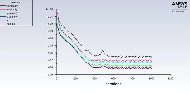
Run the solution for an estimated 1500 iterations. The convergence may occur at any intermediate step.

Results :

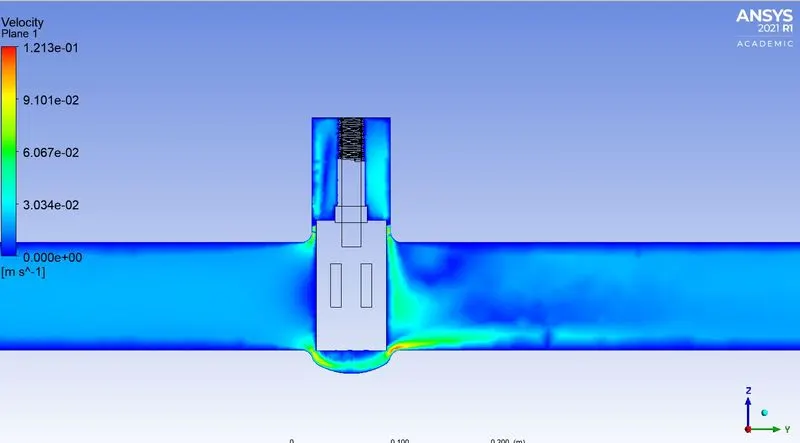
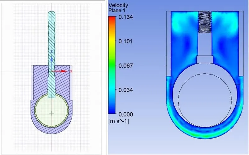
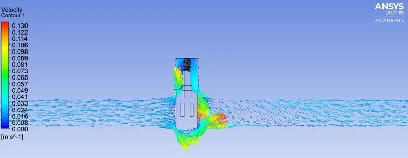
1.For a valve opening of 10 mm :

a.Residual plot :

b. Velocity contour plot :

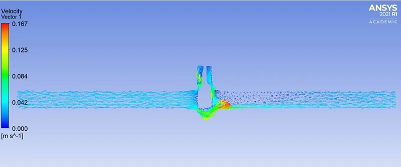
c. Velocity vector plot

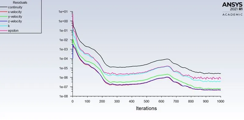
2. For a valve opening of 20 mm

a. Residual plot

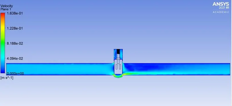
b. Velocity contour plot:

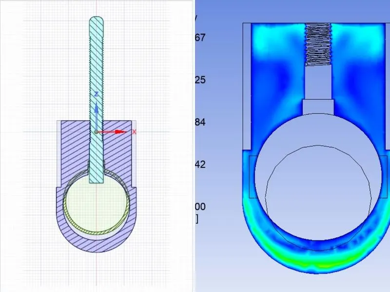
c. Velocity vector plot

3. For a valve opening of 30 mm

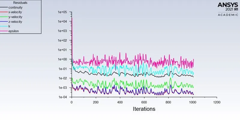
a. Residual plot :

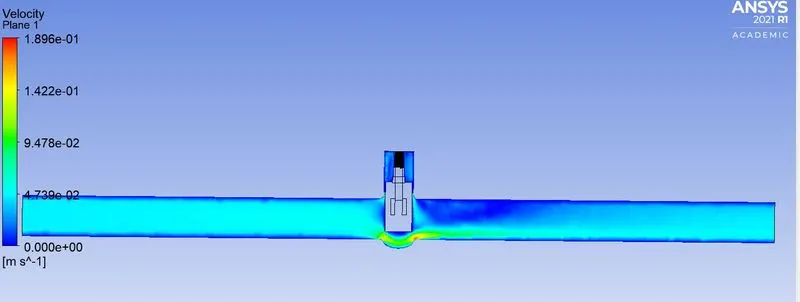
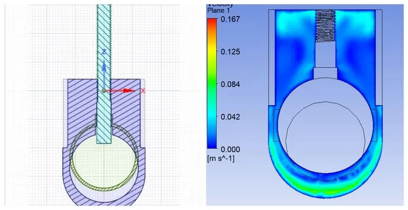
b. Velocity contour plot:

c. Velocity vector plot

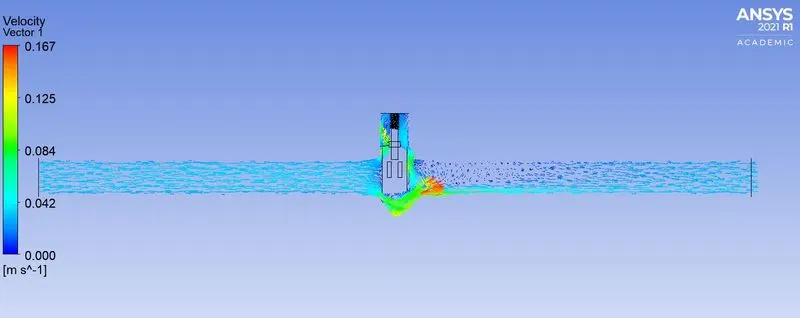
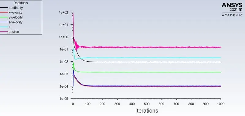
4. For a valve opening of 40mm

a. Residual plot :

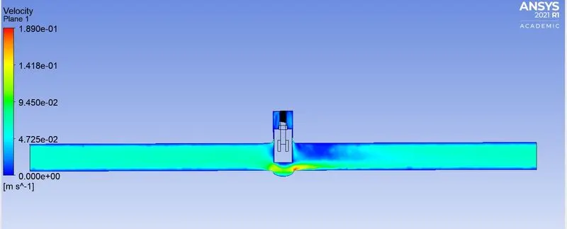
b. Velocity contour plot :

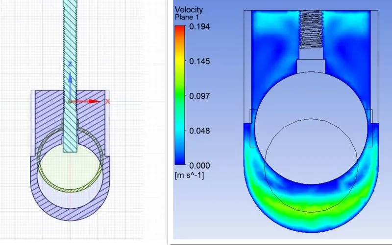
c. Velocity vector plot

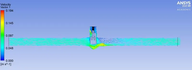
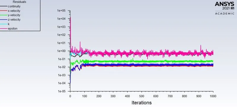
5. For a valve opening of 50 mm

a. Residual plot :

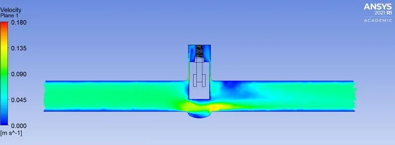
b. Velocity contour plot

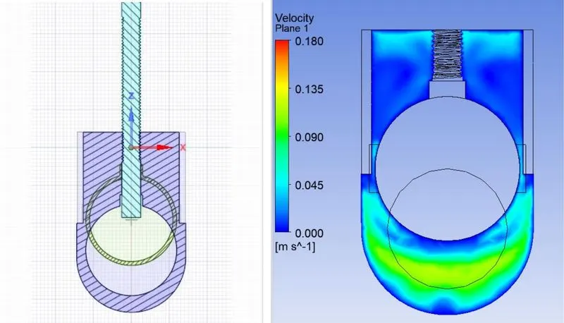
c. Velocity vector plot

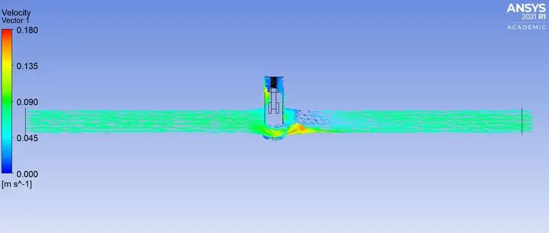
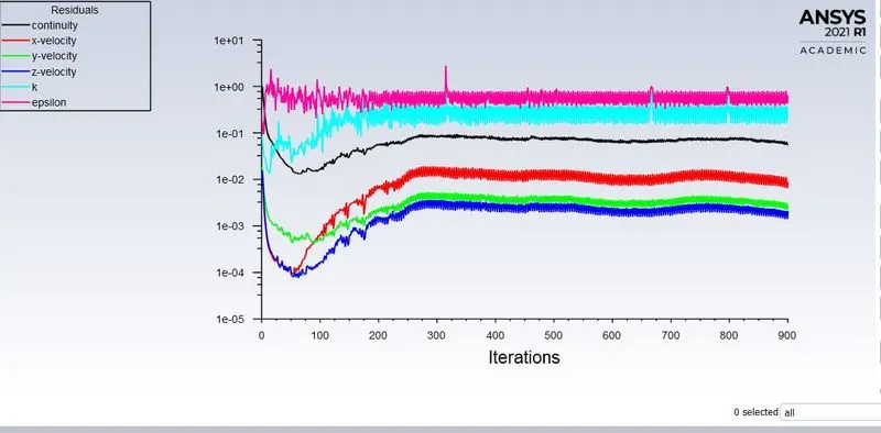
For opening of 60 mm

a. Residual plot

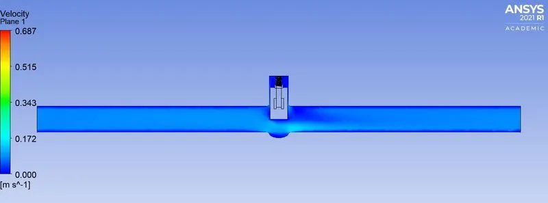
b. Velocity contour plot :

c. Velocity vector plot

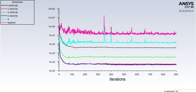
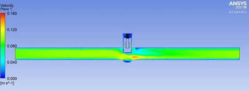
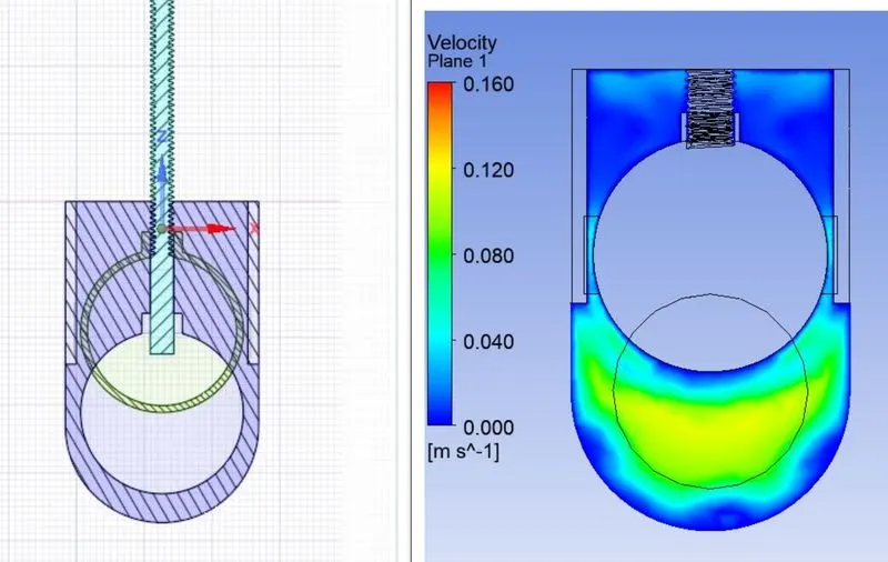
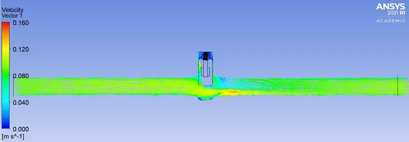
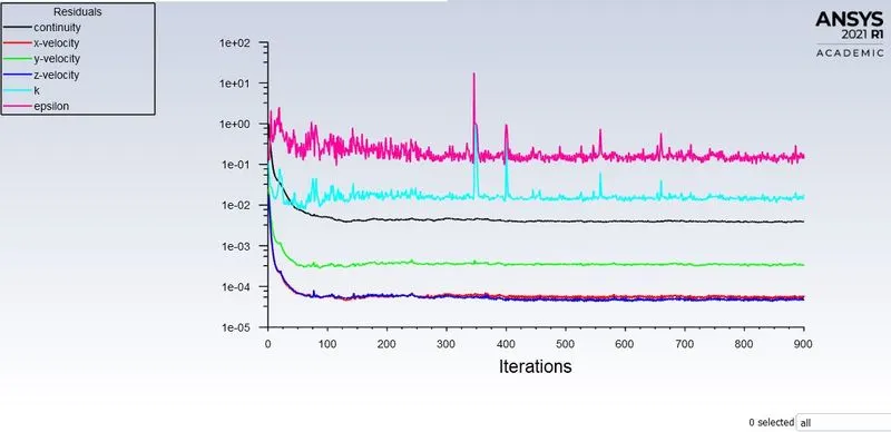
For an opening of 70 mm

a. Residuals

b. Velocity contour plot

c. Velocity vector plot

b. Velocity contour plot

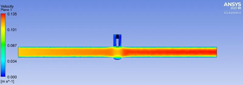
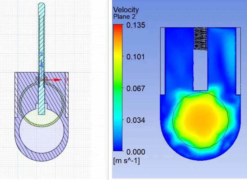
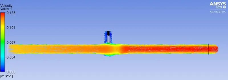
For a gate oopening of 80 mm.

a. Residuals

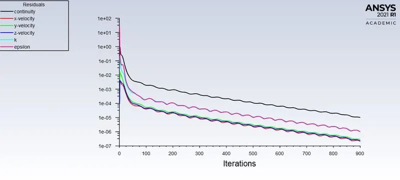
b. Velocity contour

c. Velocity vector plot

Results :

Table of Design points :

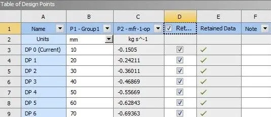
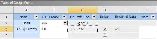
Tabular data of results :

Lift (in mm)	Mass flow rate (in kg/s)	Mass flow rate (in gallons/min)	Inlet Pressure (in Pa)	Outlet Pressure (in Pa)	`Delta`P (P in - P out)
10	-0.1505	2.3412	10	0	10
20	-0.24211	3.7561	10	0	10
30	-0.36011	5.726	10	0	10
40	-0.46869	7.4201	''	''	"
50	-0.55669	9.0858	''	''	"
60	-0.62843	9.9396	''	''	"
70	-0.69363	11.3014	''	''	"
80	-0.85297	12.0178	''	''	"

Table for the Flow coefficient (Cv) and Flow factor (Kv)

Flow coefficient (Cv)	Flow factor (Kv) Kv = 0.865 * CV
61.4829	53.1827
98.6400	85.3236
150.372	130.0717
194.861	168.5547
238.604	202.8134
261.026	225.7875
296.789	256.723
315.603	272.996

Graphical interpretation of the Flow coefficient (Cv) and Flow factor (Kv) :

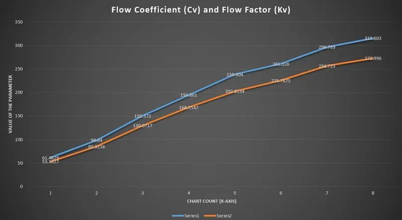
The data in the blue curve and red curve represents the Flow coefficient and Flow factor respectively.

Result analysis :

It can be seen that with an increase in the Mass flow rate the Flow coefficient (Cv) and the Flow factor (Kv) increase in a linear fashion.

This is because the mathematically `C_v = Q*(sqrt((SG)/(Delta P)))` and Cv is directly proportional to the first power of Discharge(Q).

Need for the parametruc study :

In an analysis where the variation of output parameter with respect to a set of input parameters is necessary, we make the input value(s) as a parameter. This enables the solver to directly solve for the output with change in input without the necessity of setting up the case from pre-processing. This has the benefit of saving the computational time due to reduced manual setup.

References :

1. Flow coefficient and flow factor :

1. Boysen, Herman. "k_v: what, why, how, whence?" (PDF). NONOPDF.com. Danfoss. Retrieved 21 April 2020.(https://assets.danfoss.com/documents/DOC026186467826/DOC026186467826.pdf)

2. Gate Valve and its components : Wikipedia, (https://en.wikipedia.org/wiki/Gate_valve#:~:text=A%20gate%20valve%2C%20also%20known,the%20gate%20is%20fully%20opened.)