Week 3 - Solving second order ODEs

An OCTAVE program that solves the differential equation governing the motion of a simple pendulum with damping and animates the path of the bob.

Background study :

A simple pendulum consists of a bob(sphere) tied to a massless string/rod (mass of the string/rod is negligible compared to the mass of the bob, Mb >>>Mt), suspended from a fixed support. The length of the thread is l.

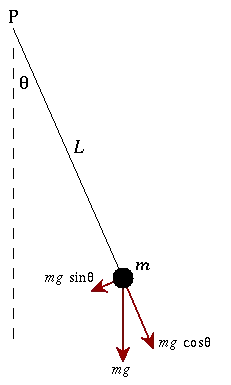
The coordinates of the pivot point P are (0,0). θ is the angular displacement of the bob which varies with respect to time and hence θ is a function of time θ(t). The coordinates of the bob for any given value of the angular displacement (θ) is given by (x,y) = `(l*sintheta, -l*costheta)`.

Note : θ is measured in radians.

The differential equation that gives the acceleration of pendulum with damping:

At any given instant of time the forces acting on the pendulum are :

Applying the Newton's second law in (`F = m * a`),

1. Along the path of the bob: (`m * a = - m * g * sintheta`) --------------(1)

'Damping force' is due to the combined damping effects of air friction and the friction at the pivot point. When the damping effect is considered, the term ' - Fd' in the Right hand side of the eqn.1 appears. The damping force has the -ve sign as it always acts in a direction which is opposite to the motion of the bob.)

The term 'a' can be written as the second derivative of the linear displacement

`a = d^2/dt x`. Here 'x' is the linear displacement.

The relation between the arc length (s), radius of the circle (l) and the angular displacement θ is given by:

s = l * θ and hence `a = d^2/dt^2 s = l (d^2/dt^2 theta)` -----------------(2).

Substitution 'a' for `l (d^2/ dt^2 theta)` gives `d^2/dt^2 s = (g/l)* sin(theta)` -------(3).

Now, the introduction of damping force which is proportional to the angular velocity (`d/dt (theta)`) in the eqn.3 gives the following equation:

`d^2/ dt^2 theta = -(b/m)*d/dt theta - (g/l)*sintheta` `--------(4)

Linearization of the differential equation :

The differential equation `d^2/dt^2 theta = -(b/m)*(d/dttheta) - (g/l)*sintheta` `

is unsuitable to solve it numerically. Hence it requires ' linearization ' - A process through which the higher order terms of the differential equation are converted into linear terms.

Steps for the linearization of equation 4:

1. Let (`theta = theta_1`) --------------(a)

2. Then ( `d/dt theta = d/dt theta_1 = theta_2`) ---------(b`

3. `d^2/dt^2 theta = d^2/dt^2theta_1 = d/dt theta_2`----- --------(c)

Substituting the relations (a),(b) and (c) in the differential equations gives us

`d/dt theta_2 = -(b/m)*theta_2 - (g/l)*sintheta_1`

In the matrix notation,

`d/dt[[theta_1],[theta_2]] = [[theta_2],[-(b/m*theta_2 + (g/l)*sintheta_1)]]`

The ODE45 solver :

The ODE45 solver solves the non-stiff (https://en.wikipedia.org/wiki/Stiff_equation) differential equations.

Consider a differential equation `d/dt y = f(t,y)`

The ode45 solver integrates the above differential equation from t_start to t_end with the available initial condition `y_0`

Syntax :

`[tsol, ysol] = ode45(@ (t,y) odefunction(t,y), t_span, y_0 )`

here, t_sol and y_sol are the solution vectors. For every value of the t_sol there is a corresponding y_sol.

ode_function = This is the function which solves the differntial eqaution and returns the solution

t_span = specifies the values of t_start and t_end over which the integration should be performed.

`y_0` = initial value of the dependent variable that corresponds to t_start.

Algorithm :

1. Define the constants damping coefficient(b), length of the string(l), mass of the bob(m) and accln. due to gravity (g).
2. Define the initial conditions of displacement and velocity as theta_0.
3. Define the time period as t_span over which the integration is performed.
4. Write an expression which uses the ode45 solver to solve the non-stiff differential equation and returns the output 'result'.
5. Use the subplot function to plot the displacement vs time; velocity vs time curves and Angular velocity vs time in a separate windows of the same plot window.
6. In order to create the animation, use a for loop which plots the position of the bob at a given instant and thus recursively plotting the position of the bob over the given time span.
7. Store the sequential plots of the bob's position in a file using the saveas function of octave.
8. Stitch them to produce a .gif file using a third party software 'image magick'.

The following code solves the differential equation and provides the velocity and displacement as an output vector - results.

clear all
close all
clc

% Defining the constants
b = 0.2;
l = 1;
m = 1;
g = 9.81;
  
% Defining the initial conditions

theta_0 = [0;3]; % 0 represents the initial value of the displacement and 3 is the value of initial velocity

% Defining the time interval for the integration

t_span = linspace(0,20,500); % linspace()returns a row vector of 'n' number of the numerical values in between the initial and final values.

% Using the ode45 solver to solve the differential equation

[t, results] = ode45(@(t,theta) pen_solver(t,theta,b,l,m,g), t_span, theta_0);

subplot(5,4, [13,14,17,18]) 
% subplot function splits the plot window into m x n windows and sets the current axis for plotting to the location given by index.

plot(t,results(:,1),'color','g');
hold on
plot(t,results(:,2),'color','r');
axis([0 30, -5 5]);
xlabel('time in seconds');
legend('displacement','velocity','location','best');
grid on;

subplot(5,4, [15,16,19,20])

 % In our case, the plot window is split into 5 x 4 = 20 windows and the current axis is set to plot at the indices [15,16,19,20].
hold on
plot(results(:,2),results(:,1),'color','b');
xlabel('position-radians');
ylabel('angular velocity');

ct = 1;
for i = 1: length(results(:,1))
  x0 = 0;
  y0 = 0;
  
  x1 = sin(results(i,1));
  y1 = -1*cos(results(i,1));
  
  subplot(5,4,[1,2,3,4,5,6,7,8,9,10,11,12]);
  plot([-1 1],[0 0],'linewidth',2,'color','b'); % Plots the support wall to which the pendulum is suspended.

  hold on
  line([x0 x1], [y0 y1],'linewidth',2,'color','b'); % Plots the string/ rod to which the bob is attached.
  hold on;

  plot(x1,y1,'-o','markers',20,'markerfacecolor','r'); % Plots the bob in red color using the marker '-o'.
  grid on;
  axis([-1.5 1.5 -1.5 0.5])
  pause(0.0003);
  hold off
 
  snip = sprintf("Pendulum%d.png",ct); 
  saveas(1,snip);
  
  ct = ct + 1;
  
  end

The function pen_solver receives the input arguments (t,theta,b,l,m,g) when called by the main program and solves the equations and returns the output argument. The code for the function pen_solver is as follows:

function dtheta_dt = pen_solver(t, theta, b, l, m ,g)
  THETA1 = theta(1);
  THETA2 = theta(2);
  
  dtheta1_dt = THETA2;
  dtheta2_dt = -(b/m)*THETA2 - (g/l)*sin(THETA1);
  
  dtheta_dt = [dtheta1_dt; dtheta2_dt];
  
endfunction

Errors generated and steps taken to debug the errors:

1. Syntactical errors :

a. Error generated due to fault in the statement containing the syntax for ode45 solver

The error is due to the faulty syntax " [t, results] = ode45(@(t,theta) pen_solver(t,theta,b,l,m,g), theta_0, t_span);". The mistake lies at the order in which the theta_0 and t_span are typed. The correct syntax should be as follows:

[t, results] = ode45(@(t,theta) pen_solver(t,theta,b,l,m,g), t_span, theta_0);

b. Error generated due to the absence of one or more input arguments during the function call.

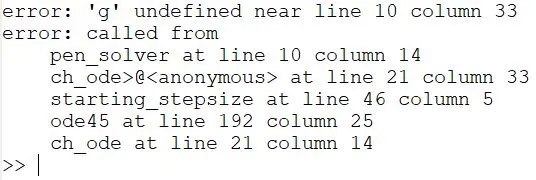
In this case the constant 'g' which is an argument to be passed as an input to the function is undefined. Defining the argument 'g' in the syntax can fix this error.

II. Semantics error : This is the type of error that is not displayed as error but diagnosed as error because the code/ logic in the code couldn't work to produce the desired output.

In this case, a fault in the initiation of the 'for loop' is the common semantics error. The possible reason(s) for this could be faults in the initiation of the loop / loop counter variable / usage of the one variable in place of others.

Output :

The output 'results' is a 500 x 2 matrix containing the values of the displacement `theta`in the first column of the matrix and the values of velocity in the second column.

Also, the .gif file which is an animation of the path of the bob is generated as output.

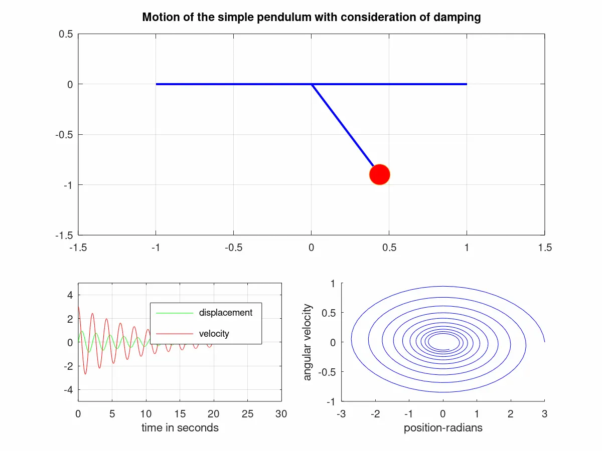
Link to the animation file : https://youtu.be/e_S4FteN5fo