Week 3 - Taylor table method and Matlab code
Taylor Table Method
Aim : To compute the fourth order approximation of the second derivative in the central,right and left schemes using the Taylor Table method.
Theory : The taylor table method is used to find the schemes with the desired accuracy and for the stencil that we choose. The taylor table method is based on the Taylor series.
Method :
Suppose that the fourth order approximation of the second derivative of a function is required i.e `f^('')`, we can proceed with any of the following schemes
I .Central scheme :
`(del^2f)/(del^2x) = a*f_(i - 2) +b*f_(i - 1) +c*f_(i ) +d*f_(i + 1) +e*f_(i + 2)`.--------(1)
The statement 1 is called the Hypothesis function.
In order to use this scheme, it is essential that we have the coefficients a,b,c,d,e and f.
Consider `f_(i + 1)` whose taylor series expansion is as follows
`f_(i + 1) = f_i + Deltax*f' + (Deltax^2)/(2!)* f'' + (Deltax^3)/(3!)*f'''+ (Deltax^4)/(4!)*f^(4) + (Deltax^5)/(5!)*f^(5) + O(Deltax^6)`
Likewise the taylor series expansion for `f_(i +2 )` looks like the above but with `Deltax` replaced by `2*Deltax`
`f_(i + 2) = f_i + 2*Deltax*f' + ((2*Deltax)^2)/(2!)* f'' + ((2*Deltax)^3)/(3!)*f'''+ ((2*Deltax)^4)/(4!)*f^(4) + ((2*Deltax^5))/(5!)*f^(5) + O(Deltax^6)`
The taylor series expansion for `f_(i -2)`looks like as follows
`f_(i - 2) = f_i - 2*Deltax*f' + ((2*Deltax)^2)/(2!)* f'' - ((2*Deltax)^3)/(3!)*f'''+ ((2*Deltax)^4)/(4!)*f^(4) - ((2*Deltax^5))/(5!)*f^(5) + O(Deltax^6)`
The Taylor series expansion for the `f_(i - 1)` is as follows
`f_(i - 1) = f_i - Deltax*f' + (Deltax^2)/(2!)* f'' - (Deltax^3)/(3!)*f'''+ (Deltax^4)/(4!)*f^(4) - (Deltax^5)/(5!)*f^(5) + O(Deltax^6)`
Tabulation of the above gives
| f' | f'' | f''' | `f^(4)` | `f^(5)` | `f^(6)` | |
| `a*f_(i -2)` | 1.a | -2.a | 2.a | -8/6.a | 16/24.a | -32/120.a |
| `b*f_(i -1)` | 1.b | -1.b | 1/2.b | -1/6.b | 1/24.b | -1/120.b |
| `c*f_(i)` | 1.c | 0 | 0 | 0 | 0 | 0 |
| `d*f_(i + 1)` | 1.d | 1.d | 1/2.d | 1/6.d | 1/24.d | 1/120.d |
| `e*f_(i +2)` | 1.e | 2.e | 2.e | 8/6.e | 16/24.e | 32/120.e |
Since it is known that the constant, first, third, fourth and fifth derivatives do not appear in the second derivative sequence, they can be equated to zero.
| `a*f_(i -2) + b*f_(i -1) + c*f_(i)+d*f_(i + 1) + e*f_(i + 2)` | 0 | 0 | 1 | 0 | 0 | 0 |
The above can be expressed in the form of a linear equation A.X = B
where A is the coefficient matrix
B is the matrix containing the values from RHS
X is the matrix containing the derivatives.
In the matrix form it can be expressed as
`[[1,-2 ,2 ,-8/6,16/24],[1,-1,1/2,-1/6,1/24],[1,0,0,0,0],[1,2,1/2,1/6,1/24],[1,2,2,8/6,16/24]]*[[a],[b],[c],[d],[e]] =[[0],[0],[1],[0],[0]]`
`X = A^(-1) * B` gives us the value of the matrix X.
Upon solving the matrix X turns out to be `[[-0.08333],[1.333],[-2.500],[1.3333],[-0.0833]]`.
Back substitution of the values obtained above into the hypothesis equation gives the final and usable form of the second order central scheme to compute the second derivative of a function.
Final Hypothesis function :
(del^2f)/(del^2x) = (-0.0833)*f_(i - 2) +(1.3333)*f_(i - 1) +(-2.5000)*f_(i ) +(1.333)*f_(i + 1) +(-0.0833)*f_(i + 2)`.--------(I)
II. Right Skewed scheme :
Consider the following Hypothesis function in the right skewed scheme:
`(del^2f)/(del^2x) = a*f_i +b*f_(i + 1) + c*f_(i + 2) + d*f_(i + 3) + e*f_(i +4)+f*f_(i + 5)`
In order to use this scheme, it is essential that we have the coefficients a,b,c,d,e and f.
Consider `f_(i + 1)` whose taylor series expansion is as follows
`f_(i + 1) = f_i + Deltax*f' + (Deltax^2)/(2!)* f'' + (Deltax^3)/(3!)*f'''+ (Deltax^4)/(4!)*f^(4) + (Deltax^5)/(5!)*f^(5) + O(Deltax^6)`
Likewise the taylor series expansion for `f_(i +2 )` looks like the above but with `Deltax` replaced by `2*Deltax`
`f_(i + 2) = f_i + 2*Deltax*f' + ((2*Deltax)^2)/(2!)* f'' + ((2*Deltax)^3)/(3!)*f'''+ ((2*Deltax)^4)/(4!)*f^(4) + ((2*Deltax^5))/(5!)*f^(5) + O(Deltax^6)`
For the `f_(i + 3)`expansion `3*Deltax`comes in the place of `Deltax`
`f_(i + 3) = f_i + 3*Deltax*f' + ((3*Deltax)^2)/(2!)* f'' + ((3*Deltax)^3)/(3!)*f'''+ ((3*Deltax)^4)/(4!)*f^(4) + ((3*Deltax^5))/(5!)*f^(5) + O(Deltax^6)`
Likewise for the `f_(i + 4)`expansion `4*Deltax`appears.
`f_(i + 4) = f_i + 4*Deltax*f' + ((4*Deltax)^2)/(2!)* f'' + ((4*Deltax)^3)/(3!)*f'''+ ((4*Deltax)^4)/(4!)*f^(4) + ((4*Deltax^5))/(5!)*f^(5) + O(Deltax^6)`
For the `f_(i + 5)`expansion `5*Deltax`appears.
`f_(i + 5) = f_i + 5*Deltax*f' + ((5*Deltax)^2)/(2!)* f'' + ((5*Deltax)^3)/(3!)*f'''+ ((5*Deltax)^4)/(4!)*f^(4) + ((5*Deltax^5))/(5!)*f^(5) + O(Deltax^6)`
Tabulation of the above gives
| f' | f'' | f''' | `f^(4)` | `f^(5)` | `f^(6)` | |
| `a*f_(i )` | 1.a | 0 | 0 | 0 | 0 | 0 |
| `b*f_(i +1)` | 1.b | 1.b | 1/2.b | 1/6.b | 1/24.b | 1/120.b |
| `c*f_(i+2)` | 1.c | 2.c | 2.c | 8/6.c | 16/24.c | 32/120.c |
| `d*f_(i + 3)` | 1.d | 3.d | 9/2.d | 9/2.d | 27/8.d | 81/40.d |
| `e*f_(i +4)` | 1.e | 4.e | 8.e | 64/6.e | 256/24.e | 1024/120.e |
| `f*f_(i +5)` | 1.f | 5.f | 25/2.f | 125/6.f | 625/24.f | 3125/120.f |
Since it is known that the constant, first, third, fourth and fifth derivatives do not appear in the second derivative sequence, they can be equated to zero.
| `a*f_(i -2) + b*f_(i -1) + c*f_(i)+d*f_(i + 1) + e*f_(i + 2)` | 0 | 0 | 1 | 0 | 0 | 0 |
The above can be expressed in the form of a linear equation A.X = B
where A is the coefficient matrix
B is the matrix containing the values from RHS
X is the matrix containing the derivatives.
In the matrix form it can be expressed as
`[[1,0,0 ,0,0,0],[1,1,1/2,1/6,1/24,1/120],[1,2,2,8/6,16/24,32/120],[1,3,9/2,9/2,27/8,81/40],[1,4,8,64/6,256/24,1024/120],[1,5,25/2,125/6,625/24,3125/120]]*[[a],[b],[c],[d],[e],[f]] =[[0],[0],[1],[0],[0],[0]]`
`X = A^(-1) * B` gives us the value of the matrix X.
upon solving the matrix X turns out to be `[[3.7500],[-12.8333],[17.8333],[-13.000],[5.0833],[-0.0833]]`
Back substitution of the values obtained above into the hypothesis equation gives the final and usable form of the second order central scheme to compute the second derivative of a function.
Final Hypothesis function :
`(del^2f)/(del^2x) = (3.7500)*f_i +(-12.8333)*f_(i + 1) + (17.8333)*f_(i + 2) + (-13.000)*f_(i + 3) + (5.0833)*f_(i +4)+(-0.8333)*f_(i + 5)`--(II)
III. Left Skewed scheme :
Consider the following Hypothesis function in the right skewed scheme:
`(del^2f)/(del^2x) = a*f_(i-5) +b*f_(i - 4) + c*f_(i - 3) + d*f_(i -2) + e*f_(i-1 )+f*f_(i )`
In order to use this scheme, it is essential that we have the coefficients a,b,c,d,e and f.
Consider `f_(i - 1)` whose taylor series expansion is as follows
`f_(i - 1) = f_i - Deltax*f' + (Deltax^2)/(2!)* f'' - (Deltax^3)/(3!)*f'''+ (Deltax^4)/(4!)*f^(4) - (Deltax^5)/(5!)*f^(5) + O(Deltax^6)`
Likewise the taylor series expansion for `f_(i +2 )` looks like the above but with `Deltax` replaced by `2*Deltax`
`f_(i - 2) = f_i - 2*Deltax*f' + ((2*Deltax)^2)/(2!)* f''- ((2*Deltax)^3)/(3!)*f'''+ ((2*Deltax)^4)/(4!)*f^(4) - ((2*Deltax^5))/(5!)*f^(5) + O(Deltax^6)`
For the `f_(i + 3)`expansion `3*Deltax`comes in the place of `Deltax`
`f_(i - 3) = f_i - 3*Deltax*f' + ((3*Deltax)^2)/(2!)* f'' - ((3*Deltax)^3)/(3!)*f'''+ ((3*Deltax)^4)/(4!)*f^(4) - ((3*Deltax^5))/(5!)*f^(5) + O(Deltax^6)`
Likewise for the `f_(i + 4)`expansion `4*Deltax`appears.
`f_(i - 4) = f_i -4*Deltax*f' + ((4*Deltax)^2)/(2!)* f'' - ((4*Deltax)^3)/(3!)*f'''+ ((4*Deltax)^4)/(4!)*f^(4)- ((4*Deltax^5))/(5!)*f^(5) + O(Deltax^6)`
For the `f_(i + 5)`expansion `5*Deltax`appears.
`f_(i - 5) = f_i - 5*Deltax*f' + ((5*Deltax)^2)/(2!)* f''- ((5*Deltax)^3)/(3!)*f'''+ ((5*Deltax)^4)/(4!)*f^(4) - ((5*Deltax^5))/(5!)*f^(5) + O(Deltax^6)`
Tabulation of the above gives
| f' | f'' | f''' | `f^(4)` | `f^(5)` | `f^(6)` | |
| `a*f_(i )` | 1.a | 0 | 0 | 0 | 0 | 0 |
| `b*f_(i -1)` | 1.b | -1.b | 1/2.b | -1/6.b | 1/24.b | -1/120.b |
| `c*f_(i-2)` | 1.c | -2.c | 2.c | -8/6.c | 16/24.c | -32/120.c |
| `d*f_(i-3)` | 1.d | -3.d | 9/2.d | -9/2.d | 27/8.d | -81/40.d |
| `e*f_(i -4)` | 1.e | -4.e | 8.e | -64/6.e | 256/24.e | -1024/120.e |
| `f*f_(i -5)` | 1.f | -5.f | 25/2.f | -125/6.f | 625/24.f | -3125/120.f |
Since it is known that the constant, first, third, fourth and fifth derivatives do not appear in the second derivative sequence, they can be equated to zero.
| `a*f_(i ) + b*f_(i -1) + c*f_(i-2)+d*f_(i -3) + e*f_(i -4)+ f*f_(i-5)` | 0 | 0 | 1 | 0 | 0 | 0 |
The above can be expressed in the form of a linear equation A.X = B
where A is the coefficient matrix
B is the matrix containing the values from RHS
X is the matrix containing the derivatives.
In the matrix form it can be expressed as
`[[1,0 ,0 ,0,0,0],[1,-1,1/2,-1/6,1/24,-1/120],[1,-2,2,-8/6,16/24,-32/120],[1,-3,9/2,-9/2,27/8,-81/40],[1,-4,8,-64/6,256/24,-1024/120],[1,-5,25/2,-125/6,625/24,-3125/120]]*[[a],[b],[c],[d],[e],[f]] =[[0],[0],[1],[0],[0],[0]]`
`X = A^(-1) * B` gives us the value of the matrix X.
Upon solving the matrix X turns out to be `[[3.75000],[-12.8333],[17.8333],[-13.0000],[5.08333],[-0.8333]]`.
Back substitution of the values obtained above into the hypothesis equation gives the final and usable form of the second order central scheme to compute the second derivative of a function.
Final Hypothesis function :
`(del^2f)/(del^2x) = (3.750)*f_i +(-12.833)*f_(i + 1) +(17.8333)*f_(i + 2) + (-13.000)*f_(i + 3) + (5.0833)*f_(i +4)+(-0.833)*f_(i + 5)`----(III)
Algorithm :
1. Define the coefficient matrices A1, A2 and A3 which represent the coefficient matrix in the equation A.X = B.
2. Also define the matrices X and B.
3. Determine the matrix X1, X2 and X3 by performing the operation `A^-1*B`.
4. Write an expression `-2*exp(x)*sin(x)`that calculates the analytical derivative of the given `f(x) = e^x*cosx`.
5. Write an anonymous function f that take the input 'x' and calculates the numerical deivative.
6. Use the expressions I, II and III to calculate the central, right skewed and left skewed derivatives.
7. Write an anonymous function g that take the input as numerical derivative values 'central_diff', 'right_skew' and 'left_skew' individually and calculates the error as the absoloute difference b/w the analytical derivative and numerical derivative.
8. Plot the dx vs error curves for the central, right skewed and left skewed schemes for comaparison.
Code :
% Creation of a taylor table

% Defining the coefficient matrix
A1 = [1 1 1 1 1;-2 -1 0 1 2; 2 1/2 0 1/2 2; -8/6 -1/6 0 1/6 8/6; 16/24 1/24 0 1/24 16/24];

A2 = [1 1 1 1 1 1;0 1 2 3 4 5;0 1/2 2 9/2 8 25/2;0 1/6 8/6 9/2 64/6 125/6; 0 1/24 16/24 27/8 256/24 625/24;0 1/120 32/120 81/40 1024/120 3125/120];

A3 = [1 1 1 1 1 1;0 -1 -2 -3 -4 -5; 0 1/2 2 9/2 8 25/2;0 -1/6 -8/6 -9/2 -64/6 -125/6;0 1/24 16/24 27/8 256/24 625/24;0 -1/120 -32/120 -81/40 -1024/120 -3125/120];

%Defining the residual matrix

B1 = [0; 0; 1; 0; 0];
B2 = [0; 0; 1; 0; 0; 0];
B3 = [0; 0; 1; 0; 0; 0];

% Calculation of the variable matrix
X1 = A1\B1;
X2 = A2\B2;
X3 = A3\B3;

x = pi/3;
dx = linspace(pi/30,pi/300,100);

% Calculation of analytical derivative of the given function
% f(x) = exp(x) * cos*(x)
% second derivative of f(x) is -2*exp(x)*sin(x)

analytical_derivative = -2*exp(x)*sin(x);

% Defining the anonymous functions

f = @(x) exp(x).*cos(x);
g = @(f) abs(f - analytical_derivative);

% calaculation of second derivative of the given function using the central
% differencing scheme,Right side skewed scheme and left side skewed
% schemes respectively.

%Central differencing scheme
central_diff = (X1(1)*f(x - 2*dx) + X1(2)*f(x - dx) + X1(3)*f(x) + X1(4)*f(x + dx) + X1(5)*f(x + 2*dx))./dx.^2;

% Right skewed scheme
right_skewed = (X2(1)*f(x) + X2(2)*f(x + dx) + X2(3)*f(x + 2*dx) + X2(4).*f(x + 3*dx) + X2(5)*f(x + 4*dx) + X2(6)*f(x + 5*dx))./dx.^2;

%Left skewed scheme
left_skewed = (X3(1)*f(x) + X3(2)*f(x - dx) + X3(3)*f(x - 2*dx) + X3(4)*f(x - 3*dx) + X2(5)*f(x - 4*dx) + X3(6)*f(x - 5*dx))./dx.^2;

%Calculation of errors
error_central = g(central_diff);
error_right = g(right_skewed);
error_left = g(left_skewed);

%plotting the errors
loglog(dx,error_central);
hold on
loglog(dx,error_right);
loglog(dx,error_left);
xlabel('range of values of dx');
legend('error central','error right','error left');
Result(s) :
I. Grid size dx vs error graphs
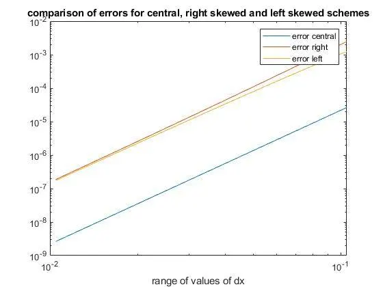
Result analysis :
Consider the following grid
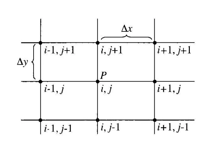
If we were to calculate the property value at grid points at the corners - `(i -1,j + 1), (i + 1, j + 1), (i - 1,j -1) and (i + 1, j -1)`, it would not have been possible by the central scheme as it requires the which are at the either sides of the grid point in consideration.
To be precise, the calculation of the property value at grid point (i - 1,j + 1) requires the property values at (i -2, j + 1) and (i + 1, j + 1). In this case the grid point (i -2, j + 1) doesn't exist.
However, the usage of the right skewed and left skewed schemes wherever appropriate will provide us the required property values at the grid points at the extremes.