Week 5 - Mid term project - Solving the steady and unsteady 2D heat conduction problem
Aim : Solving the steady and unsteady 2D heat conduction equation.
Objectives : 1. To use the Jacobian, Gauss Seidel and Successive Order Relaxation iterative techniques to the steady state 2D heat
heat conduction equation
2. To use the iterative techniques to solver the transient 2D heat conduction equation.
3. To present the CFL criteria for the explicit schemes.
Theory :
The need for iterative methods :
Consider a linear system of discretized differential equations of the form `A.X = B`
Here, A is the coefficient matrix
X is the matrix of unknown quantities and
B is the RHS values of the linear equation.
The usual way of solving these differential equations is through one of the direct methods :
1. Cramer's rule and
2. Gaussian elimination
However if the matrix is of million cells, it will be computationally expensive (requiring more time or usage of parallel solvers) using the direct methods.
However, if we employ the iterative schemes like
1. Jacobi Method
2. Gauss Seidel method or
3. Successive Over Relaxation (SOR) iteration methods the complexity can be reduced.
These iterative schemes are based on the initial guess value and the initial value is used for obtaining the next set of values. The iteration method comes to convergence when the values from two successive iteration do not differ by a prefixed tolerance value.
Mathematically, `||u^(k+1) - u^(k)|| <=epsilon`
where `u^(k+1) and u^(k)`are the values at k + 1 th and k th iteration respectively.
`epsilon`is the tolerance.
The 2D heat conduction equation without the source terms in the steady state is given by the formula:
`(del^2T)/(delx^2) + (del^2T)/(dely^2) = 0`
The discretized linear equation in the second order central scheme is :
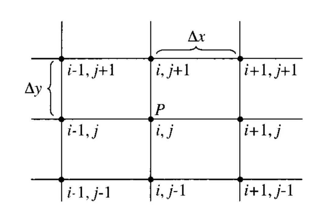
`(T_(i+1,j) - 2T_(i,j) + T_(i-1,j) )/(Deltax^2) + (T_(i,j+1) - 2T_(i,j) + T_(i,j-1) )/(Deltay^2)`
In order to compute the `T_(i,j)` i.e., the temperature at point P let the term `T_(i,j)` be shifted to the left hand side of the equation.
`T_(i,j) = (T_(i+1,j) + T_(i-1,j) + T_(i,j+1) + T_(i,j-1))/ 4`.
For a grid spacing of 1 unit in both the X and Y directions the Heat conduction equation is solved.
For solving the given problem the boundary conditions mentioned are considered
Temperature at the extreme left = 400K
Temperature at the extreme right = 800K
Temperature at the extreme top = 600K
Temperature at the extreme bottom = 900K
To simulate the Heat conduction problem the following logic is implemented:
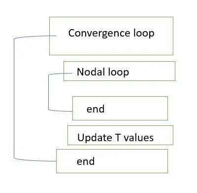
Algorithm :
1. Create a nx by ny sized matrix which represents the grid for the computation. Here nx and ny are the number of nodes in x and y directions respectively.
2. Create a nx by ny sized array T of ones and multiply it with 300 as it serves the initial guess for the temperature values at the nodes. Assign the boundary temperaures to the extreme nodes.
3. Consider the grid spacing to be unity in both the x and y directions.
4. Create a matrix t_old whose elements are same as those the matrix T. Matrix serves the purpose of the variable whose values get updated after every iteration in space.
5. Define a variable error which initially has a large numeric value say `9*e^9`. Also declare a variable called tolerance whose value is `1*e^-4`.
6. Create a loop control structure which executes the nodal loop as long as the loop criteria statement is valid. Thus the loop terminates once the criteria is failed which in our case is the error value falling below the tolerance value. This is an indication of convergence.
* Convergence : In numerical methods, convergence is the phenomenon when the change in the property value for two successive iterations is almost equal to zero.
Jacobi iterative technique :
Consider the discretized 2D heat conduction equation
`T_(i,j)^(k+1) = (T_(i+1,j)^(k) + T_(i-1,j)^(k) + T_(i,j+1)^(k) + T_(i,j-1)^(k))/ 4`
This iteration technique uses the values of the property obtained after the first iteration to calculate the values of that property before the second iteration.
In our case, to compute the values of the Temperature at `k + 1`th iteration, the values of T at the k th iteration are used.
Gauss Seidel iteration technique :
Instead of using the property values from the previous iteration, the terms calculated during the current iteration are used to compute the property value at the current iteration.
`T_(i,j)^(k+1) = (T_(i+1,j)^(k + 1) + T_(i-1,j)^(k + 1) + T_(i,j+1)^(k+ 1) + T_(i,j-1)^(k+1))/ 4`.
Here, the values `T_(i-1,j)^(k + 1) and T_(i,j-1)^(k + 1)` which belong to the current time step `k +1`are used in the calculation of `T_(i,j)^(k + 1)`.
This would help the solution to converge faster as the updated values are used in the computation.
Successive over relaxation technique :
The successive over relaxation (SOR) is a variation of Gauss Siedel method for solving the linear system of equations resulting in the faster convergence.
The formula for SOR is
`T_(i,j)^(k+1) = alpha((T_(i+1,j)^(k+1) + T_(i-1,j)^(k+1) + T_(i,j+ 1)^(k+1) + T_(i,j-1)^(k+1))/4) + (1-alpha)*T_(i,j)^k`
In the above formula `alpha`is called the relaxation factor. If the Jacobi/ Gauss Seidel method pushes the old approximation towards the original solution by 1 unit, the SOR method pushes by `alpha` times. However, a greater value of `alpha`can overshoot which would instead diverge the solution instead of converging.
Hence a relaxation factor `1 leq alpha leq 2`must be chosen as the sprectral radius `rho(L_omega) <1` for this limits of relaxation factor.
Code :
I . 2D steady heat conduction - Implicit scheme
% A program to simulate the 2D transient heat conduction in the cartesian
% coordinates

clear; close all;clc

% Creating the 2D grid with the given boundary conditions
T_H = 1:1:9;
T_V = 9:-1:1;
t  = 300*ones(1,9);
TT = meshgrid(t);
TT(1,:) = 600; TT(end,:) = 900; TT(2:end - 1,1) = 400; TT(2:end - 1,end) = 800;
TT(1,1) = 500 ; TT(1,end) = 700 ; TT(end,1) = 650 ; TT(end,end) = 850;
t_old = TT;
t = TT;
t_ini = TT;

list = menu('Types of iteration schemes available','Jacobian','Gauss-Seidel','Successive Over Relaxation');

% Defining the grid spacing and time spacing
dx = 0.1; dy = 0.1; dt = 0.1;
%a = 1.4; % alpha value for Aluminium at 0 degree centigrade

% The temperature at grind point (i,j) in the 2D grid can be computed
% using the formula :
% t(i,j) = 0.25*((t(i+1,j)+ t(i-1,j)+t(i,j+1)+t(i,j-1))

error = 9e9;
tol = 1e-4;
iter = 0;
iterative_solver = 2;

switch list

    case 1
        fprintf('Steady state 2D heat conduction using Jacobian iteration technique \n');
while (error > tol)

    for i = 2: length(TT) - 1
        for j = 2 : length(TT) - 1
            t(i,j) = 0.25*((t(i+1,j)+ t(i-1,j)+t(i,j+1)+t(i,j-1)));
        end
    end
    error = max(max(abs(t - t_old)));
    t_old = t;
    iter = iter + 1;
    contourf(T_H,T_V',t,'ShowText','ON')
    title('Steady state 2D heat conduction using Jacobian iteration technique');
    colorbar
    pause(0.02)
    iter = iter + 1;
end
fprintf('Total number of iterations = %d \n',iter);
    case 2
        fprintf('Steady state 2D heat conduction using Gauss Seidel iteration technique \n');
        while (error > tol)
        for i = 2: length(TT) - 1
            for j = 2 :length(TT) - 1
                t(i,j) = 0.25*(t(i+1,j) + t(i - 1,j) + t(i,j+1) + t(i,j -1));
            end
        end
        error  = max(max(abs(t - t_old)));
        t_old = t;
        contourf(T_H,T_V,t,'ShowText','ON');
         title('Steady state 2D heat conduction using Gauss Seidel iteration technique');
    colorbar
    pause(0.02)
    iter = iter + 1;
        end
         fprintf('Total number of iterations = %d \n',iter);

    case 3
        fprintf('Steady state 2D heat conduction using Successive over Relaxation technique \n')
        rf = input('Please enter the relaxation factor : ');
         while (error > tol)
        for i = 2: length(TT) - 1
            for j = 2 :length(TT) - 1
                t(i,j) = 0.25*(t(i+1,j) + t(i - 1,j) + t(i,j+1) + t(i,j -1));
                t_rf = (rf*t) + (1 - rf)*(t);
            end
        end
        error  = max(max(abs(t_rf - t_old)));
        t_old = t_rf;
        contourf(T_H,T_V,t,'ShowText','ON');
         title('Steady state 2D heat conduction using Gauss Seidel iteration technique');
    colorbar
    pause(0.02)
    iter = iter + 1;
        end
         fprintf('Total number of iterations = %d \n',iter);

end
Plots :
1. 2D Steady state head conduction using the Jacobian iterative scheme
- Using the Jacobian iteration technique
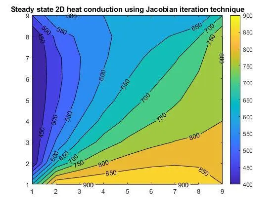
It took 178 iterations to converge.
b. Gauss Siedel iteration technique
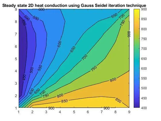
It took 89 iterations to converge.
c. Successive Over relaxation technique
For `omega` = 1
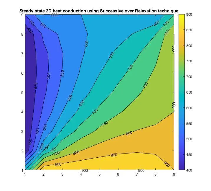
It took 89 iterations to converge.
For `omega` = 1.25
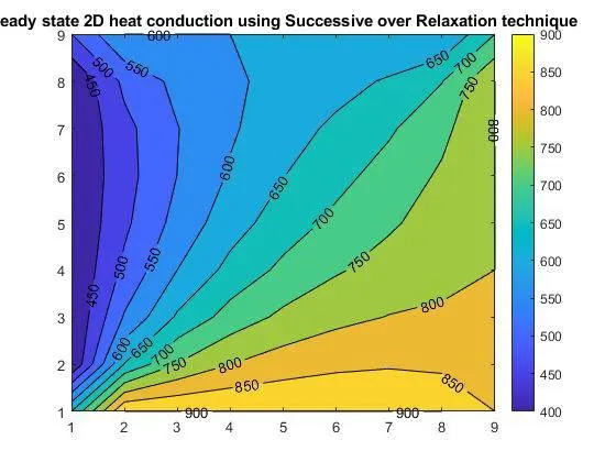
It took 78 iterations to converge.
For `omega` = 1.5
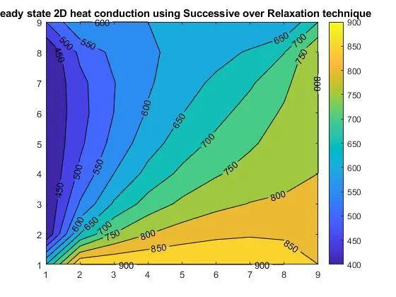
It took 66 iterations to converge.
For `omega`= 1.6
It took 60 iterations to converge.
For `omega` = 1.75
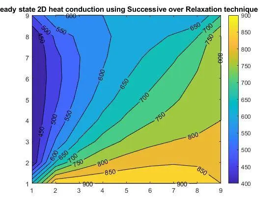
It took 39 iterations to converge.
For `omega` = 1.8
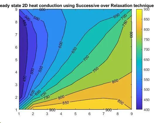
It took 43 iterations to converge.
By observation it can be stated that the best relaxation factor for this problem is 1.75 and the values starting from 1.65 through 1.8 can be used for better results.
Result analysis :
For 2D steady state analysis :
| Method employed | CFL number | `omega` | Number of iterations |
| Jacobi | N.A | N.A | 178 |
| Gauss Seidel | N.A | N.A | 89 |
| Successive Order Relaxation | N.A | 1 | 89 |
| 1.25 | 78 | ||
| 1.5 | 66 | ||
| 1.6 | 60 | ||
| 1.75 | 39 | ||
| 1.8 | 43 |
The explicit schemes provide the result faster than implicit schemes however they are bound to the CFL stability criteria. A CFL number of less than or equal to guarantees the stability for the explicit schemes.
If the `omega` (SOR) factor becomes 1, then the result provided by the SOR method will be same as that of the Gauss Seidel method.
Transient Heat Conduction:
The transient heat conduction is different to steady system in a way that the temperature of the system changes with the time and it will reach a steady state after sufficiently long time.
The 2D transient heat conduction equation is as follows :
`(delT)/(delt) = alpha((del^2T)/(del^2x) + (del^2T)/(del^2y))`
The discretized equation of the above with `Deltax, Deltay and Delta t`as grid spacing in the x and y directions respectively and the value of the time step.
`(T_(curent) - T_(old))/(Deltat) = alpha*((T_T - 2*T_p + T_B)/(Deltay^2)+ (T_R - 2*T_p + T_L)/(Deltax^2))`
Considering (i,j) as the current grid position the above equation can be written as
`(T_(i,j)^(n+1) - T_(i,j)^(n))/(Deltat) = alpha*((T_(i+1,j) - 2*T_(i,j) + T_(i-1,j))/(Deltax^2) + (T_(i,j+1) - 2*T_(i,j) + T_(i,j-1))/(Deltay^2))`
I. 2D Transient heat conduction in the explicit scheme
In the explicit scheme, the values in the right hand side of the equation are from the previous time step and hence are known. So the `T_(i,j)^(n+1)` term which is at (n+1) th time step is unknown and has to be determined. Isolating the `T_(i,j)^(n+1)` term to the LHS we obtain
`T_(i,j)^(n+1) = T_(i,j)^n+ alpha*Deltat((T_(i+1,j) - 2*T_(i,j) + T_(i-1,j))/(Deltax^2) + (T_(i,j+1) - 2*T_(i,j) + T_(i,j-1))/(Deltay^2))`
Further simplifying the above equation we obtain
`T_(i,j)^(n+1) = T_(i,j)^n(1 - (2*alpha*Deltat)/(Deltax^2) -(2*alpha*Deltat)/(Deltay^2) )+ alpha*Deltat((T_(i+1,j) + T_(i-1,j))/(Deltax^2) + (T_(i,j+1) + T_(i,j-1))/(Deltay^2))`
Let `k1 = (alpha*Deltat)/(Deltax^2)` and `k2 = (alpha*Deltat)/(Deltay^2)`.
From the values in the previous time step i.e at (`n th`) iteration, the valuesin the current time step (n + 1) can be easily calculated.
CFL criteria for stability :
For the explicit schemes
`(alpha*Deltat)/(Deltax^2) + (alpha*Deltat)/(Deltay^2) <= 0.5`.
The vaules of the `alpha, Deltat , Deltax and Deltay` should be carefully selected the the CFL criteria is obeyed for the solution to converge. Else the solution will blow up and will never converge.
Algorithm :
1. Create a nx by ny sized matrix which represents the grid for the computation. Here nx and ny are the number of nodes in x and y directions respectively.
2. Create a nx by ny sized array T of ones and multiply it with 300 as it serves the initial guess for the temperature values at the nodes. Assign the boundary temperaures to the extreme nodes.
3. Consider the grid spacing to be unity in both the x and y directions.
4. Create a matrix t_old whose elements are same as those the matrix T. Matrix serves the purpose of the variable whose values get updated after every iteration in space.
5. Define a variable error which initially has a large numeric value say `9*e^9`. Also declare a variable called tolerance whose value is `1*e^-4`.
6. Create a loop control structure which executes the nodal loop as long as the loop criteria statement is valid. Thus the loop terminates once the criteria is failed which in our case is the error value falling below the tolerance value.
7. Create a time loop which runs as long as the convergence is achieved.The nodal loop is placed inside the time loop. As a result, the nodal loop executes the statements till the error falls below the tolerance at that time step. The loop breaks and error value is agian initiated to 9e9. Thus the nodal loop executes for the next time step. The loop runs as long as the convergence is achieved.
* Convergence : In numerical methods, convergence is the phenomenon when the change in the property value for two successive iterations is almost equal to zero.
Code for the 2D Transient heat conduction in the explicit scheme :
% % A program to simulate the 2D transient heat conduction in cartesian coordinates

clear; close all;clc

% Creating a 2D grid with the boundary conditions

T = 300*ones(9,9);

T(1,1) = 500; T(1,2:end - 1) = 600; T(1,end) = 700;
T(2:end-1,:) = 400 ;T(2:end -1,end) = 800;
T(end,1) =650; T(end,2:end - 1) = 900; T(end,end) = 850;

t_old = T;
t_prev = T;
t = T;

% Defining the grid spacing and time spacing
dx = 0.1; dy = 0.1; dt = 0.1;
a = 1e-4;

% Defining the terms required for computation of temperature profile
k1 = a*dt/(dx^2);
k2 = a*dt/(dy^2);

term1 = (1 - 2*k1 - 2*k2)^-1;
term2 = k1*term1;
term3 = k2*term1;

error = 9e9;
convergence = 9e9;
tol = 1e-4;

%Running the simulation

iter = 0;
while(convergence > 1e-4)

for i = 2:length(T) - 1
    for j = 2:length(T) -1
        h = (t_old(i -1,j) + t_old(i + 1,j));
        v = (t_old(i,j - 1) + t_old(i,j + 1));
        t(i,j) = (t_prev(i,j)*term1) - (h*term2) - (v*term3);
    end
end
t_old = t;
contourf(flipud(t),'ShowText','ON');
text_line = sprintf('time iterations = %d',iter);
title(text_line);
pause(0.01)
convergence = max(max(abs(t_prev - t)));
iter = iter + 1;
t_prev = t;
error = 9e9;
end
Plots :
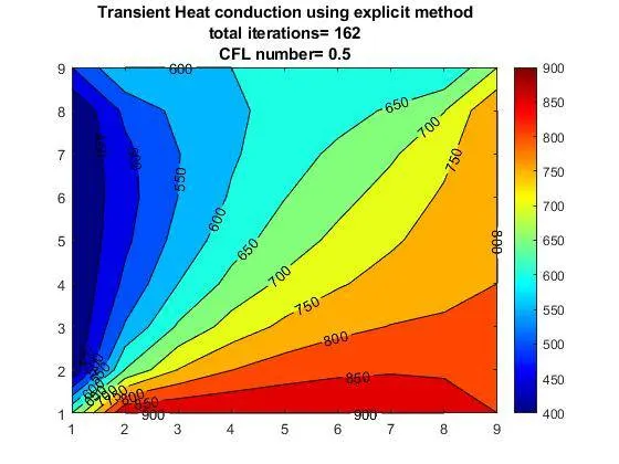
2D Transient Heat conduction equation using the explicit scheme.
II. 2D Transient heat conduction using the implicit scheme
In the RHS of the explicit scheme, the property values at the previous time step are used for computation.
Instead if we were to take values of the property at the previous nodes and at the current time step i.e (n + 1)th as and when they are determined, then it is called Implicit scheme.
This scheme improves the accuracy of the solution.
`T_(i,j)^(n+1)= T_(i,j)^(n)+alpha*Deltat*((T_(i+1,j)^(n+1) - 2*T_(i,j)^(n+1) + T_(i-1,j)^(n+1))/(Deltax^2) + (T_(i,j+1)^(n+1) - 2*T_(i,j)^(n+1) + T_(i,j-1)^(n+1))/(Deltay^2))`
Further simplifying it we obtain
`T_(i,j)^(n+1)*(1 + (alpha*Deltat)/(Deltax^2) + (alpha*Deltat)/(Deltax^2) )= T_(i,j)^(n)+alpha*Deltat*((T_(i+1,j)^(n+1) + T_(i-1,j)^(n+1))/(Deltax^2) + (T_(i,j+1)^(n+1) + T_(i,j-1)^(n+1))/(Deltay^2))`
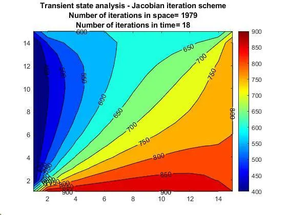
- Jacobian iterattive technique
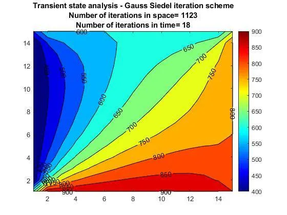
b. Gauss Seidel iteration technique
c. Successive Order Relaxation
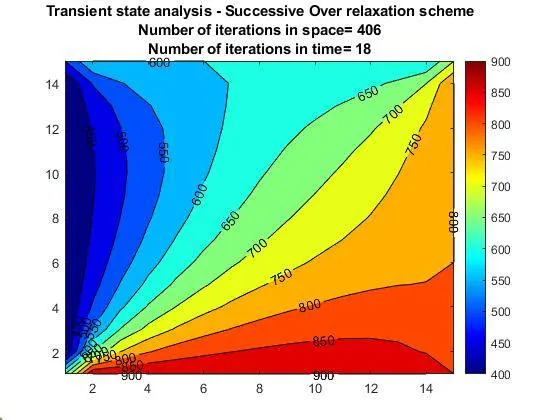
For `omega` = 1.5
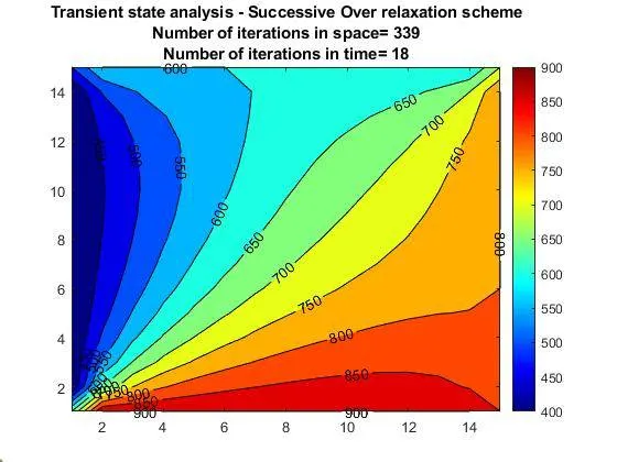
For `omega` = 1.6
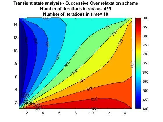
For `omega` = 1.7
Result analysis :
Transient 2D Heat conduction - explicit vs implicit
| Type of the scheme | Iteration scheme | CFL number | `omega` | Number of iterations |
| Explicit | N.A | 0.5 | 162 | |
| Implicit | Jacobi Iterative scheme | N.A | 1979 | |
| Implicit | Gauss Siedel Iterative scheme | N.A | 1123 | |
| Implicit | Succesive Over Relaxation | N.A | 1.5 | 406 |
| '' | N.A | 1.6 | 338 | |
| '' | N.A | 1.7 | 425 |
The explicit schemes provide the solution faster compared to the implicit schemes. However, the explicit schemes are not unconditionally stable as the implicit schemes are.
The CFL criteria which determines the stability of the explicit schemes has to be taken into account while employing the explicit schemes.
A CFL number of `alpha*(dt/(dx^2) + dt/(dy^2)) leq 0.5` should be checked for before proceeding for running the solver.
Though the implicit schemes are unconditionally stable, they do not converge faster. Hence we take the advantage of iterative techniques like Jacobi, Gauss-Siedel and Successive Over Relaxation for obtaining the solution faster.
It can be observed that the Gauss Seidel Technique provides the solution faster than the Jacobi technique as it uses the values obtained at the same iteration to compute the next property value.
But compared to Jacobi and Gauss Seidel techniques the SOR scheme provides the solution even faster provided the value of `omega` is between 1 and 2. Since the spectral radius for that particaular `omega`range is `leq`1 .