Week 9 - Parametric study on Gate valve.

Parametric study on Gate valve

AIM:

• Perform a parametric study on the gate valve simulation by setting the opening from 10 % to 80%.

OBJECTIVE:

• Obtain the mass flow rates at the outlet for each design point.
• Calculate the flow coefficient and flow factor for each opening and plot the graph.
• Discuss the results of the mass flow rate and flow coefficient.

THEORY:

Gate valves

A gate valve is the most common type of in-line valve used for opening and closing the flow of water in a pipeline. It has a function to stop or allow the flow. It is not used to regulate flow. It is also known as a sluice valve. A component slides into the flow stream to provide shutoff and acts as a gate. That is why it is called a gate valve. The primary objective of installing a gate valve is to isolate or shut off certain areas of the mainline for maintenance, repair work, and new installation. It can be also used to reroute the flow in a pipeline.

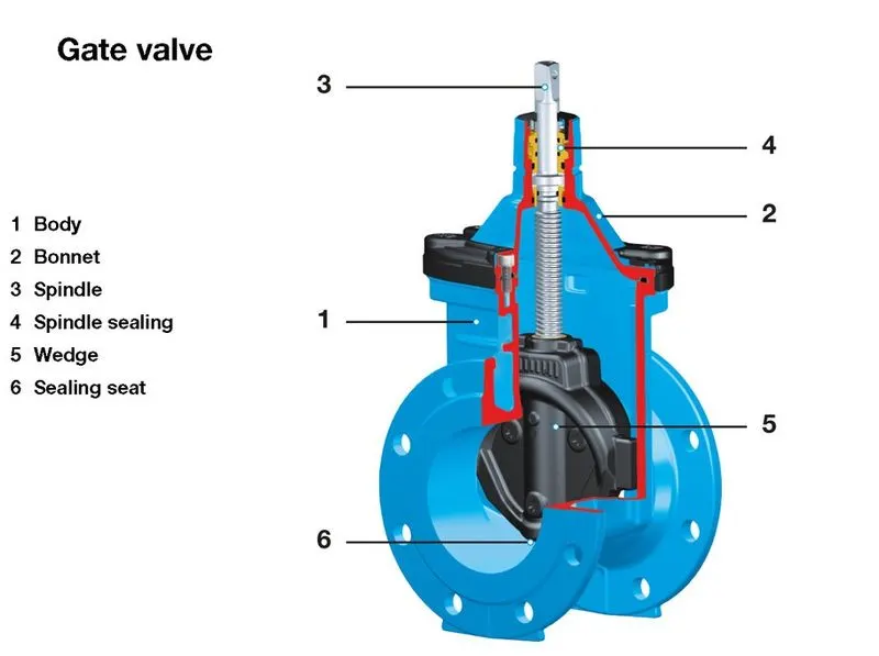
Our main objective in this challenge is to conduct a parametric study. We have chosen a gate valve for that purpose as we can adjust the linear movement of the stem and disc.

Flow Coefficient (Cv)

The flow coefficient gives us an idea about the sizing of the valve according to the flow requirements. It is important as it will affect the hydraulic efficiency of the entire pipeline. It is technically defined as “the volume of water at 60°F (in US gallons) that will flow through a valve per minute with a pressure drop of 1 psi across the valve.”

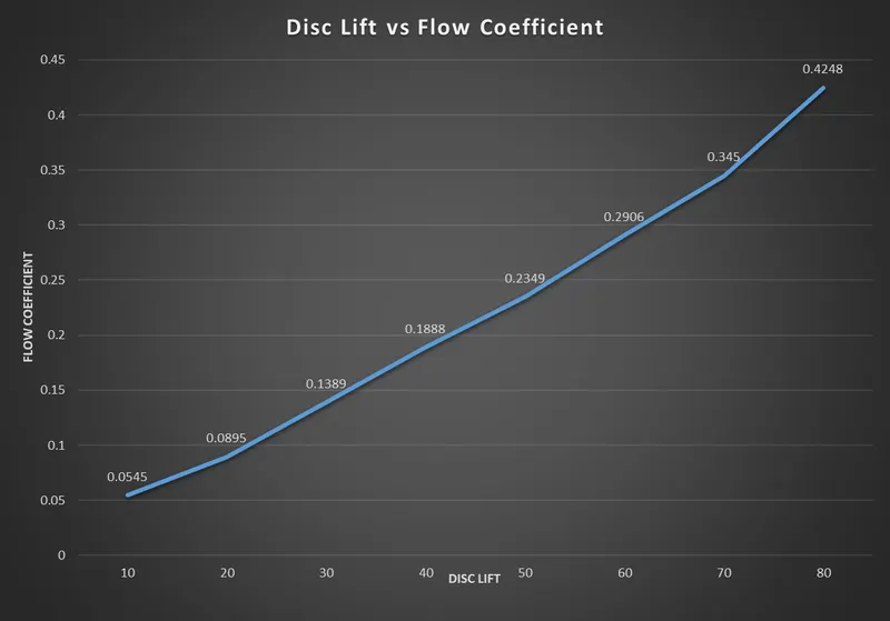
In simple terms, we can say that the larger the valve opening, the higher the value of the flow coefficient. When the valve is fully opened, the value of the flow coefficient will reach its maximum value (100% or 1).

`C_v = Qsqrt((SG)/(grad P))`

Flow factor (K_v)

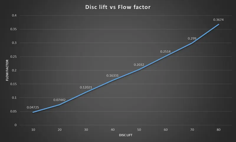
It is the metric equivalent of the flow coefficient. It is the flow of water with a temperature ranging from 5 - 30 ^oC through a valve in cubic meters per hour (m³/h) with a pressure drop of 1 bar.

`K_v = 0.865 *C_v`

PREPROCESSING:

Geometry

• Import the model to Spaceclaim.

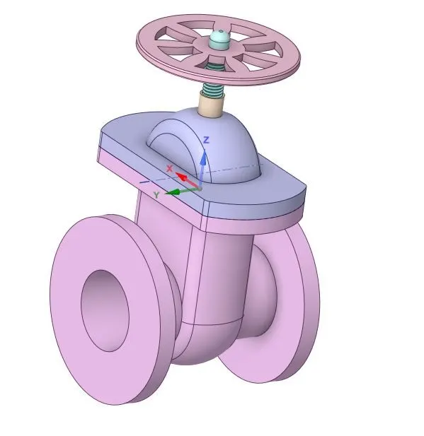
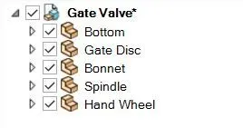
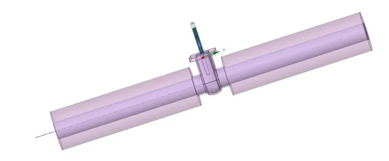
• Now extend the inlet and outlet by 800 mm by using the Pull command.

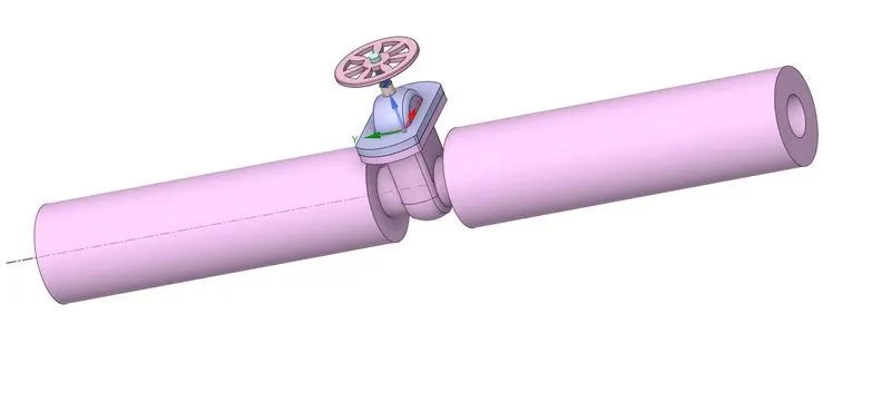
• Use the Extract tool to extract the fluid volume.

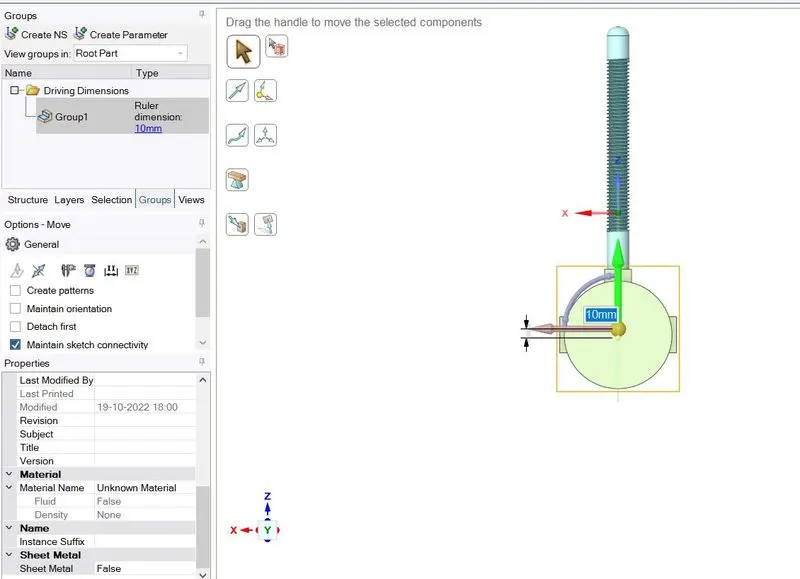
• Now we have to parameterize the lift of the valve. For that hide all other components and display only the gate disc and spindle.
• Use the Move tool under the Design tab and then select 'Move Component'. Select the Gate disc. Now the coordinate system will appear and select the direction in which the gate has to be moved. Give the distance as 10 mm.

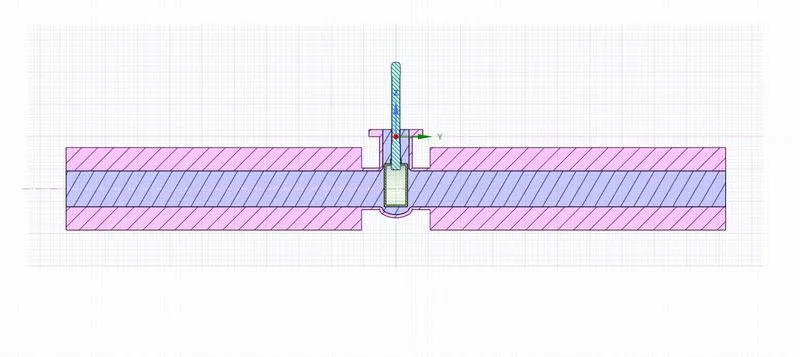
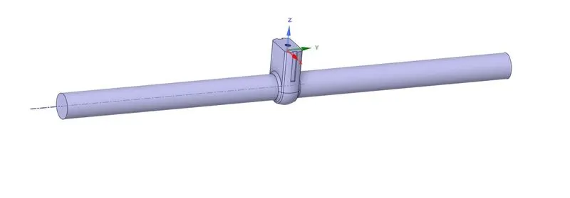
• Use the 'Suppress for Physics' option on the solid components so that it won't interfere with the simulation.

Meshing:

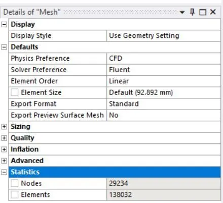
• Mesh is generated using default settings and the mesh element size is set as 50mm.

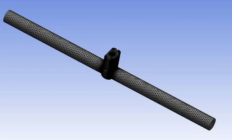
• The number of mesh elements is 138032

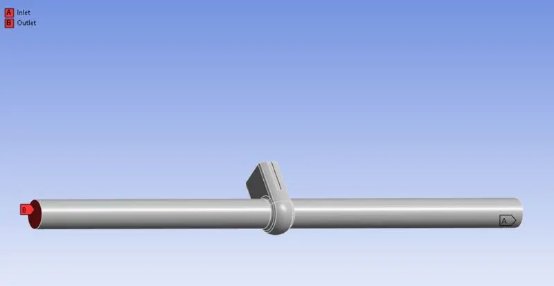
• Assign names for inlet and outlet using the 'Create named selection' option

Fluent Setup

1.	Solver Type	Pressure Based
2.	Solver Time	Steady State
3.	Gravity	Enabled (-9.81m/s^2 in z-direction)
4.	Viscous Model	K epsilon RNG with Swirl movement enabled
5.	Material	Water
6.	Input Parameter	Lift of the gate valve
7.	Output Parameter	Mass flow rate at the outlet
8.	Inlet and Outlet	Pressure Outlet

• Assign the inlet total pressure as 20 Pa.
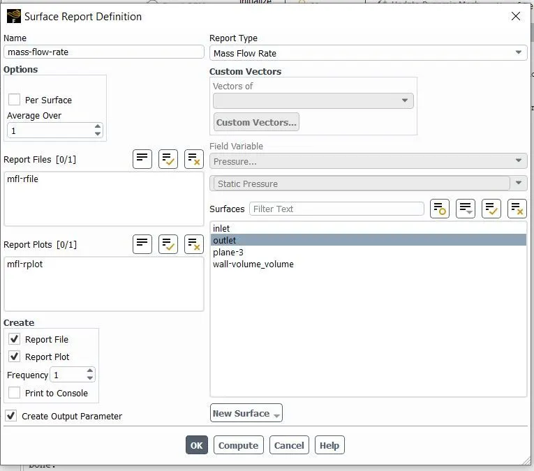
• Give a Surface Report Definition for the mass flow rate at the outlet. Use the 'Create Output Parameter' option to assign the output parameter.

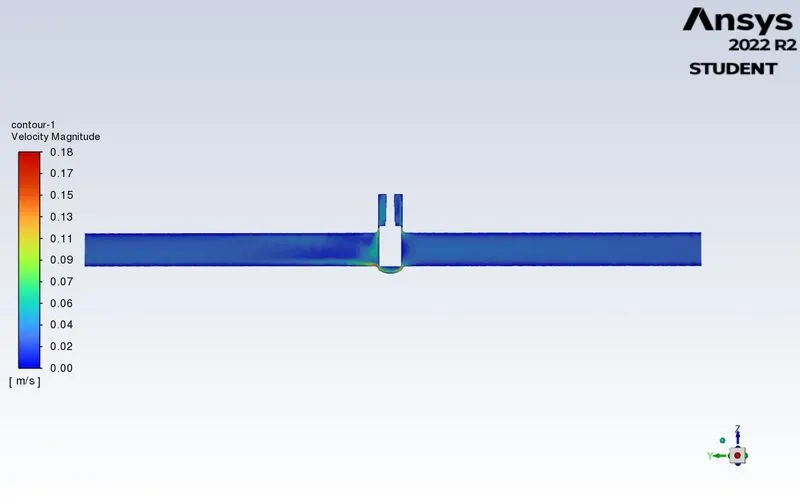
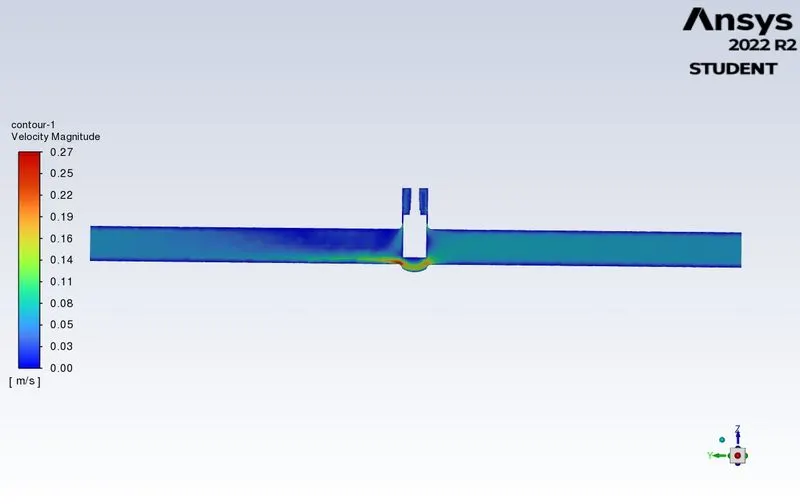
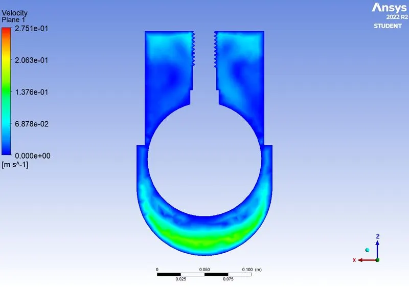
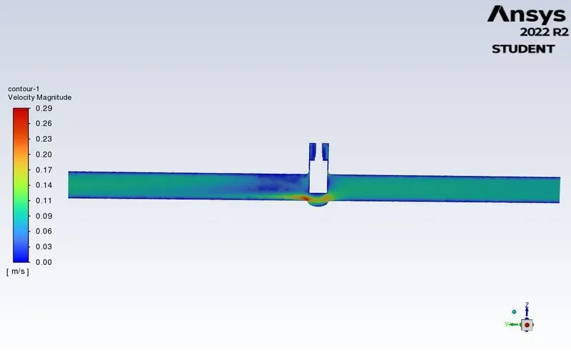
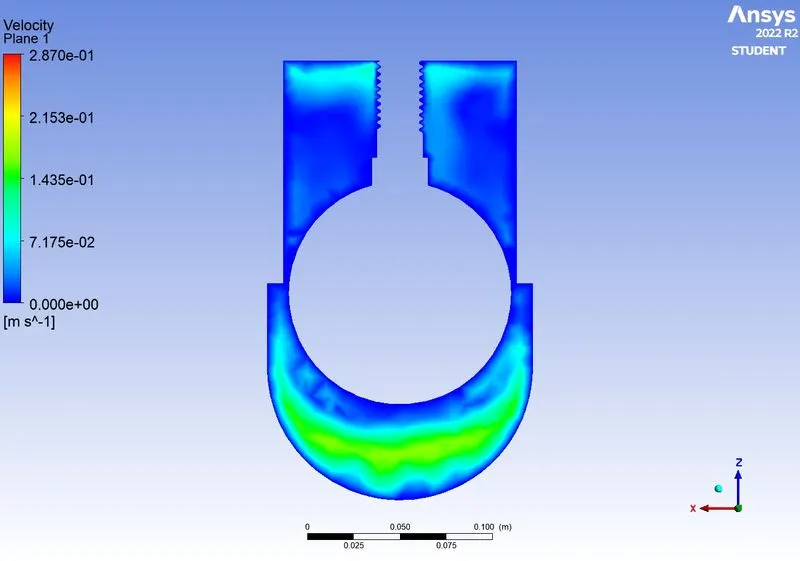
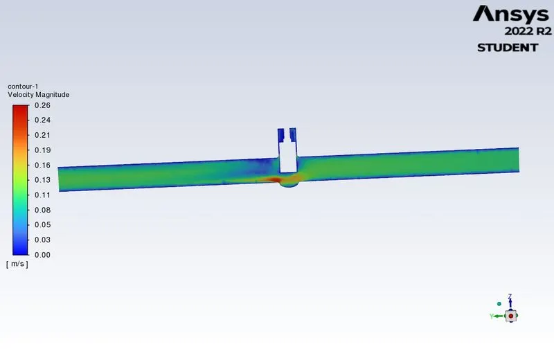
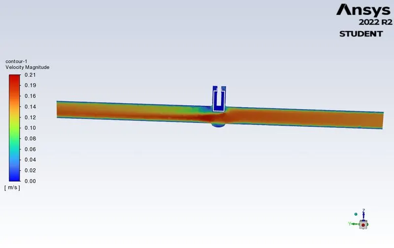
• Create a reference plane in the YZ direction and a velocity contour is created on that plane.
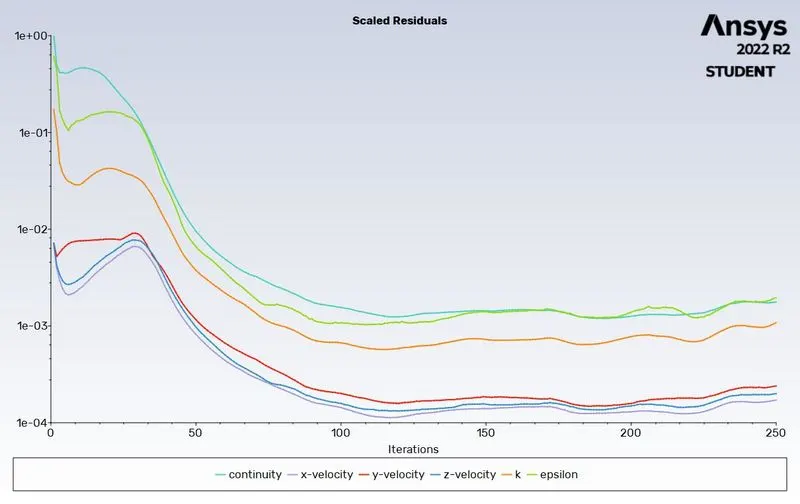
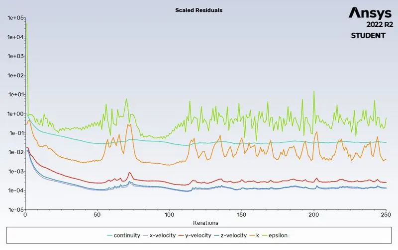
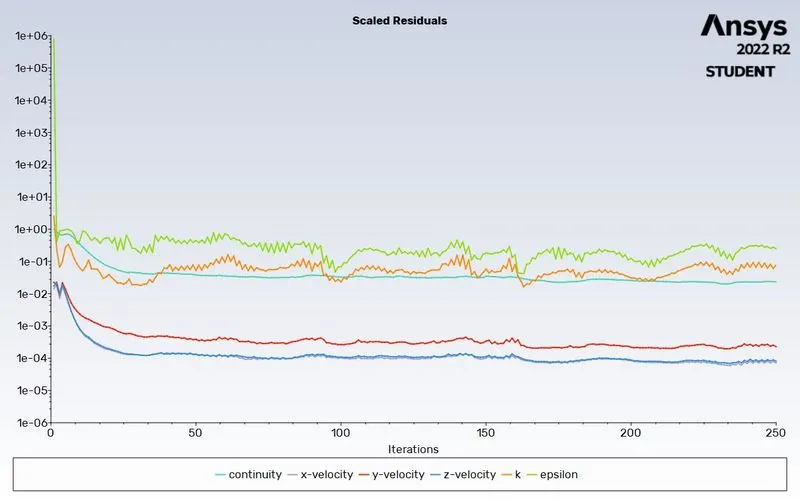
• After Hybrid initialization, run the simulation for 250 iterations.

RESULTS:

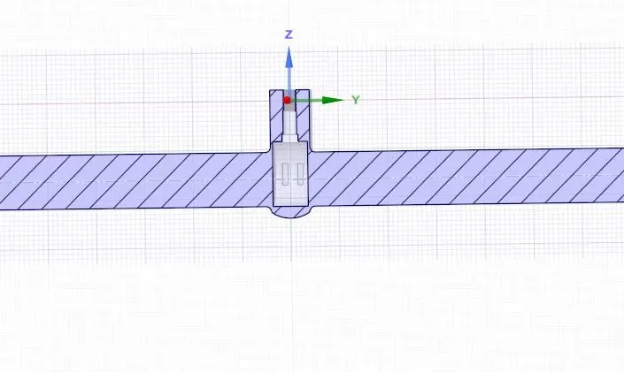
Case 1 (10 mm lift)

• Geometry

• Residuals

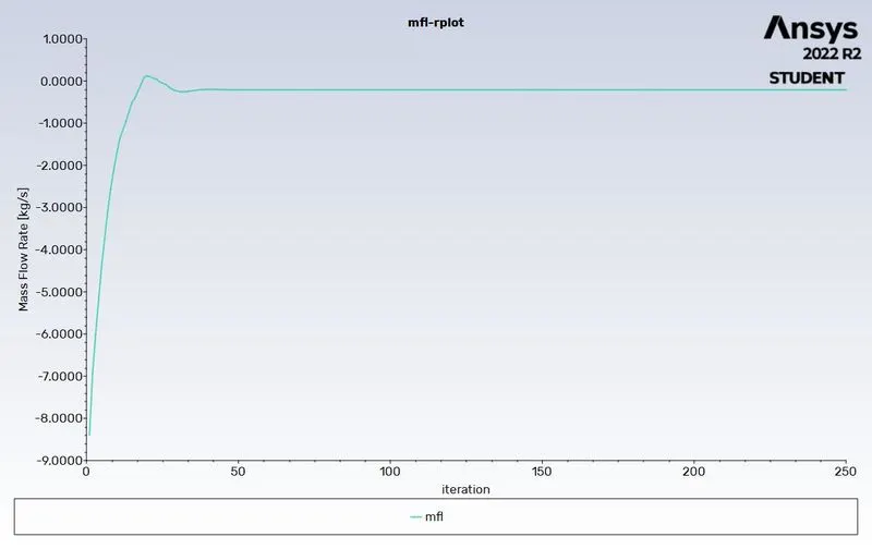
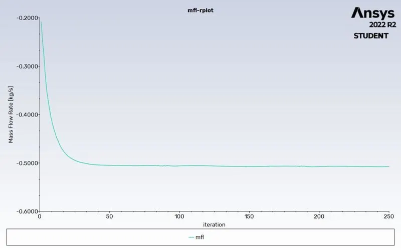
• Mass flow rate

• Velocity contour (YZ direction)

• Velocity contour (XZ direction)

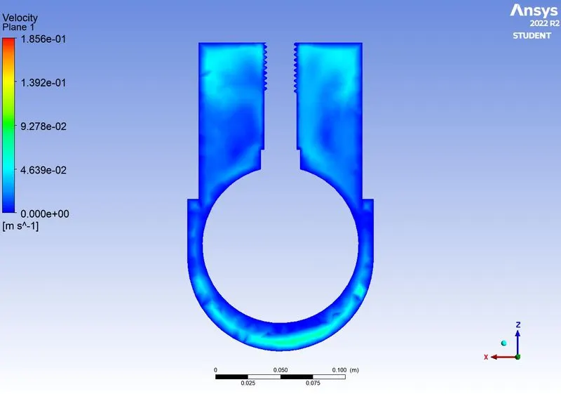
Case 2 (20 mm lift)

• Geometry

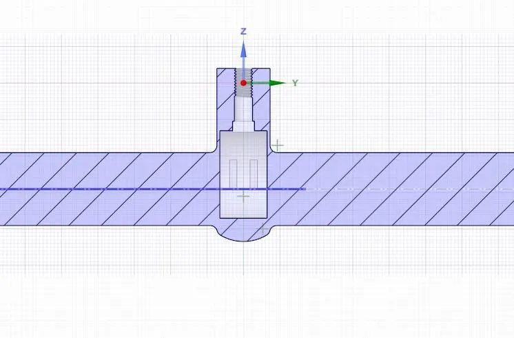
• Residuals

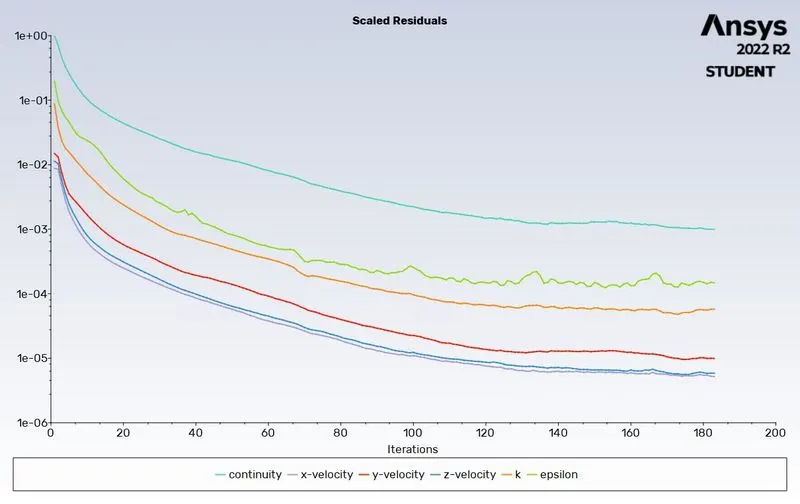
• Mass flow rate

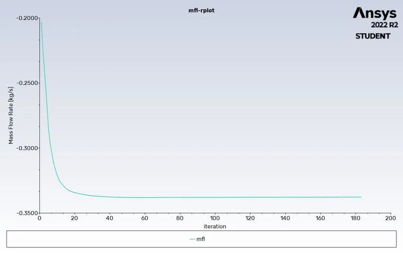
• Velocity contour (YZ direction)

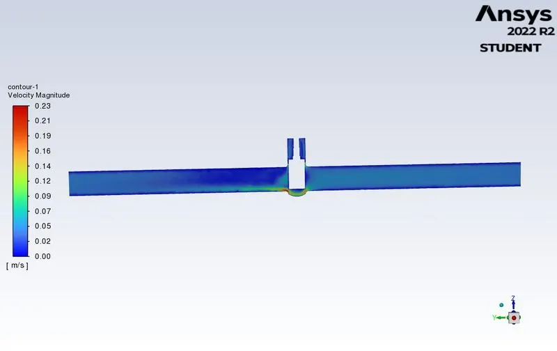
• Velocity contour (XZ direction)

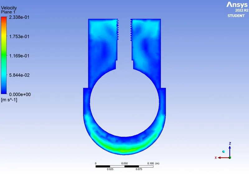
Case 3 (30 mm lift)

• Geometry

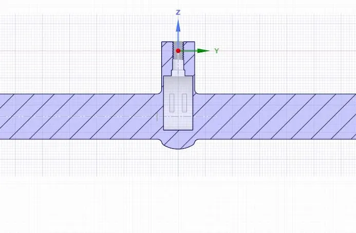
• Residuals

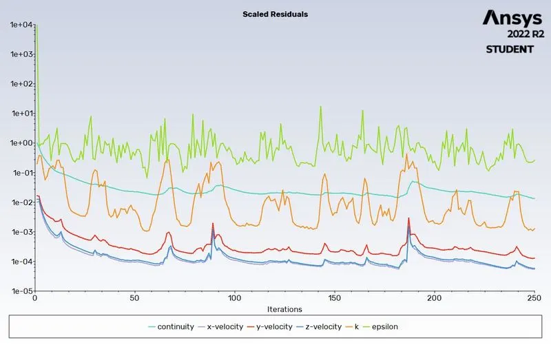
• Mass flow rate

• Velocity contour (YZ direction)

• Velocity contour (XZ direction)

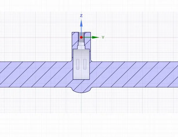
Case 4 (40 mm lift)

• Geometry

• Residuals

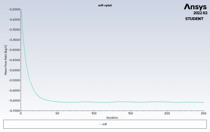
• Mass flow rate

• Velocity contour (YZ direction)

• Velocity contour (XZ direction)

Case 5 (50 mm lift)

• Geometry

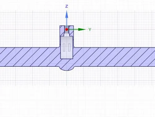
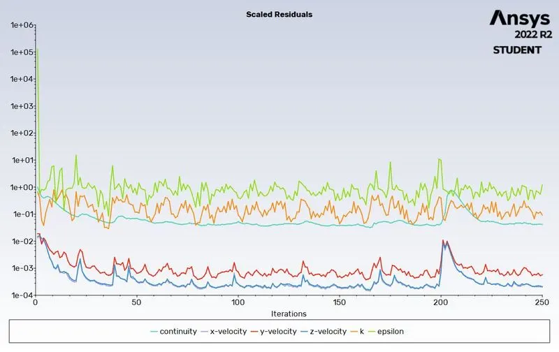
• Residuals

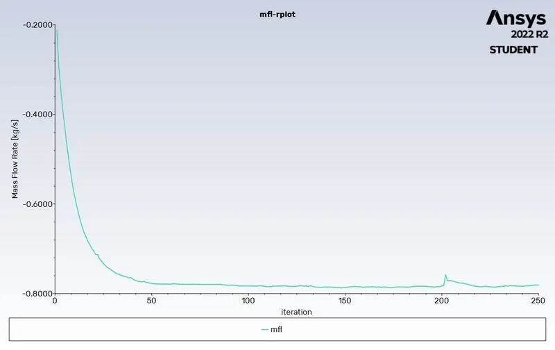
• Mass flow rate

• Velocity contour (YZ direction)

• Velocity contour (XZ direction)

Case 6 (60 mm lift)

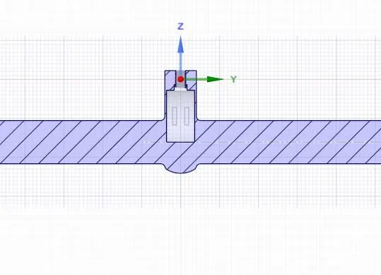
• Geometry

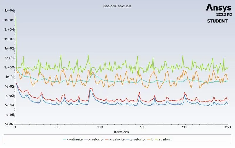
• Residuals

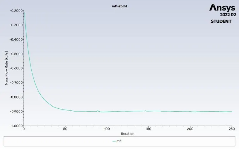
• Mass flow rate

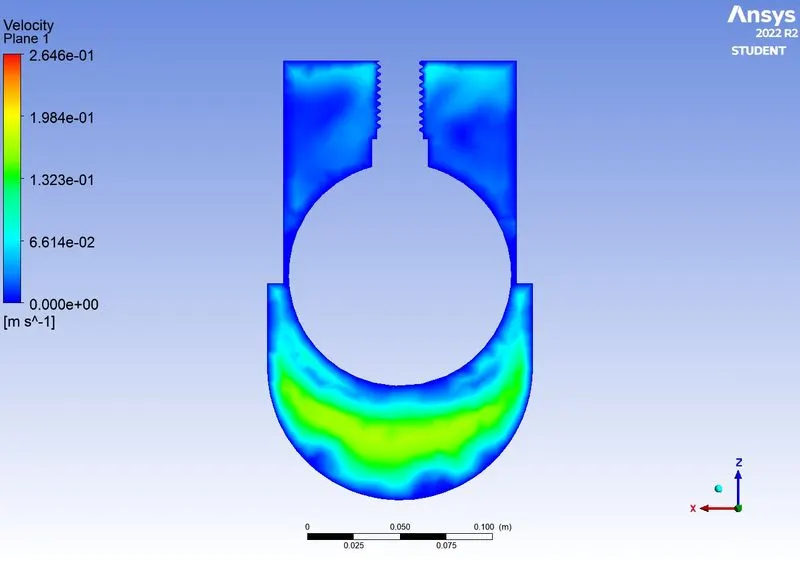
• Velocity contour (YZ direction)

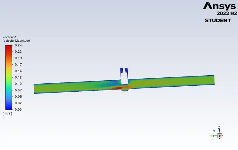
• Velocity contour (XZ direction)

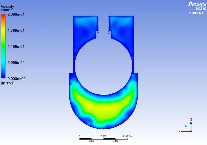
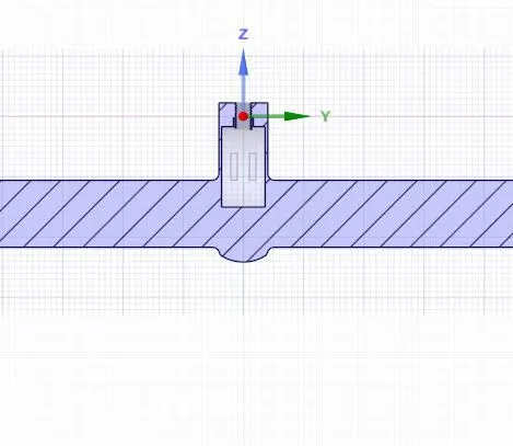
Case 7 (70 mm lift)

• Geometry

• Residuals

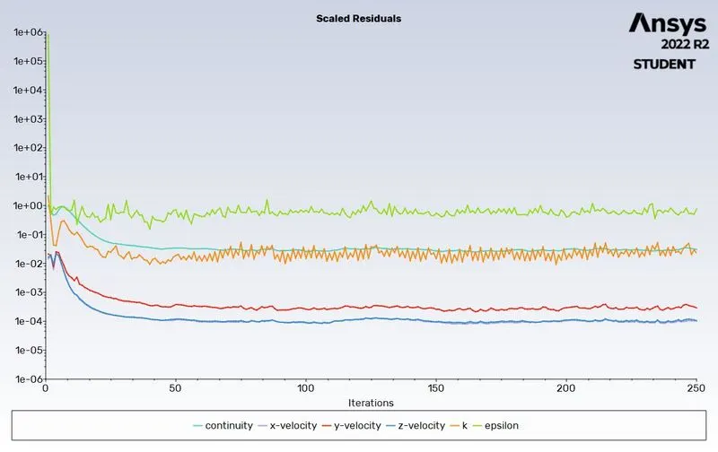
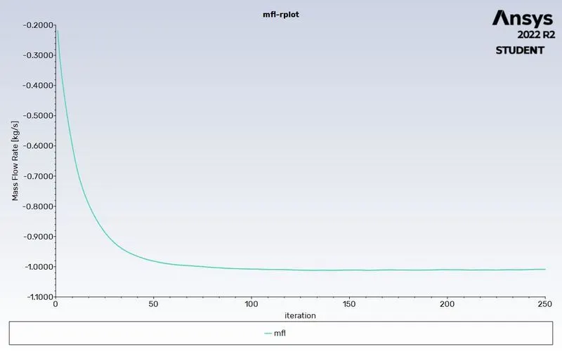
• Mass flow rate

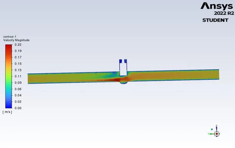
• Velocity contour (YZ direction)

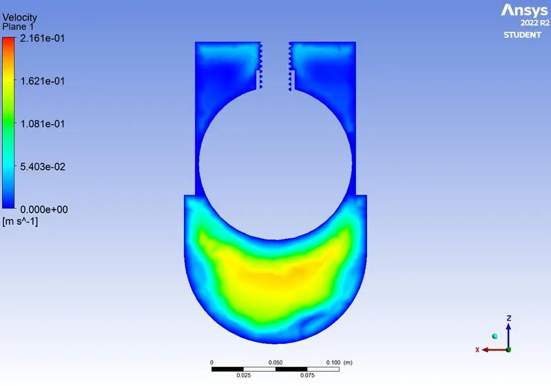
• Velocity contour (XZ direction)

Case 8 (80 mm lift)

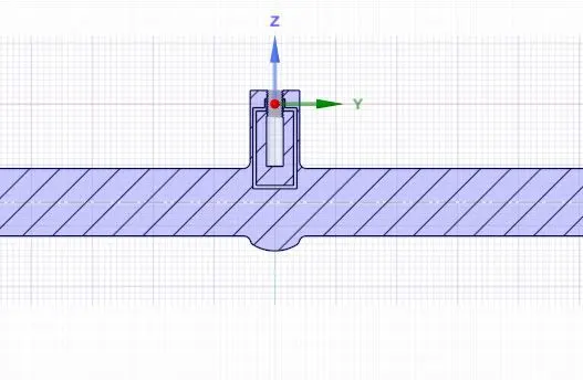
• Geometry

• Residuals

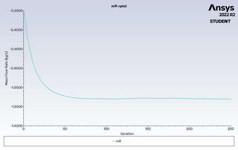
• Mass flow rate

• Velocity contour (YZ direction)

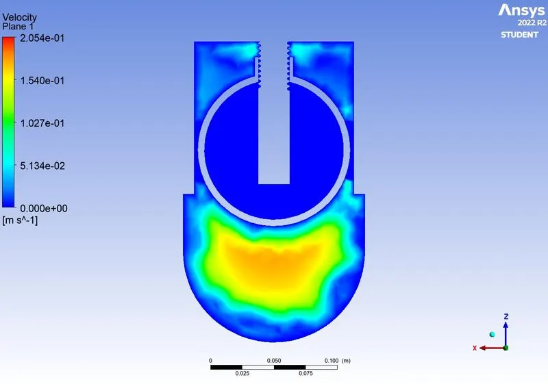
• Velocity contour (XZ direction)

Plots and Comparison Table

• Flow coefficient plot

• Flow factor plot

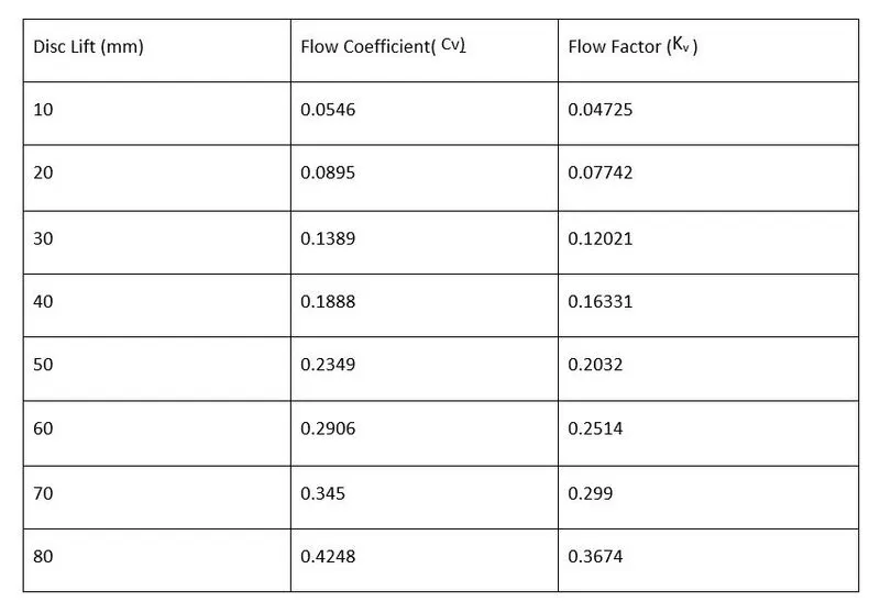
• Table

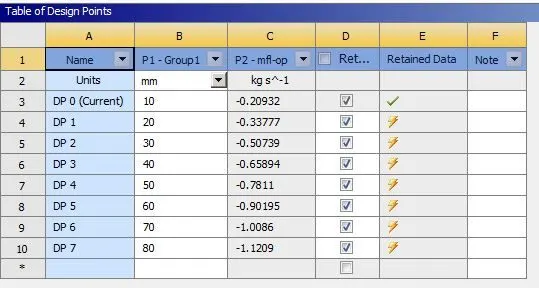
• Mass Flow Rate

CONCLUSIONS:

1. As the value of the disc lift is increased, the mass flow rate at the outlet also increases.
2. The value of the Flow coefficient and Flow factor is directly proportional to the mass flow rate. As the mass flow rate increases, the flow coefficient and flow factor also increase.
3. The negative sign of mass flow rate indicates that the fluid(water) is leaving the pipeline.
4. The parametric study is used in this case to save time as we don't have to conduct simulations for each case one by one.