Week 9 - Mini project - Flow over an Airfoil

Flow over an air foil

• Aim:

To perform steady and Transient simulation over a NACA 2412 Airfoil for varying angle of attacks. Calculate the co-efficient of drag and lift for different AOA using the time averaging method to find a optimum drag force and lift force. Plot the necessary contours and graphs to give a better understanding.

• Theory:

1. Angle of attack:

In fluid dynamics, angle of attack (AOA, α, or ) is the angle between a reference line on a body (often the chord line of an airfoil) and the vector representing the relative motion between the body and the fluid through which it is moving. Angle of attack is the angle between the body's reference line and the oncoming flow. This article focuses on the most common application, the angle of attack of a wing or airfoil moving through air.

In aerodynamics, angle of attack specifies the angle between the chord line of the wing of a fixed-wing aircraft and the vector representing the relative motion between the aircraft and the atmosphere. Since a wing can have twist, a chord line of the whole wing may not be definable, so an alternate reference line is simply defined. Often, the chord line of the root of the wing is chosen as the reference line. Another choice is to use a horizontal line on the fuselage as the reference line (and also as the longitudinal axis). Some authors do not use an arbitrary chord line but use the zero lift axis where, by definition, zero angle of attack corresponds to zero coefficient of lift.

- Relation between angle of attack and lift co-efficient

The lift coefficient of a fixed-wing aircraft varies with angle of attack. Increasing angle of attack is associated with increasing lift coefficient up to the maximum lift coefficient, after which lift coefficient decreases.

As the angle of attack of a fixed-wing aircraft increases, separation of the airflow from the upper surface of the wing becomes more pronounced, leading to a reduction in the rate of increase of the lift coefficient. The figure shows a typical curve for a cambered straight wing. Cambered airfoils are curved such that they generate some lift at small negative angles of attack. A symmetrical wing has zero lift at 0 degrees angle of attack. The lift curve is also influenced by the wing shape, including its airfoil section and wing planform. A swept wing has a lower, flatter curve with a higher critical angle.

2. Drag:

In fluid dynamics, drag (sometimes called air resistance, a type of friction, or fluid resistance, another type of friction or fluid friction) is a force acting opposite to the relative motion of any object moving with respect to a surrounding fluid. This can exist between two fluid layers (or surfaces) or a fluid and a solid surface. Unlike other resistive forces, such as dry friction, which are nearly independent of velocity, drag force depends on velocity.

a. Drag force:

Drag force is proportional to the velocity for a laminar flow and the squared velocity for a turbulent flow. Even though the ultimate cause of a drag is viscous friction, the turbulent drag is independent of viscosity. Drag forces always decrease fluid velocity relative to the solid object in the fluid's path.

where

Fd is the drag force,

is the density of the fluid,

is the speed of the object relative to the fluid,

is the cross sectional area, and

is the drag coefficient – a dimensionless number.

b. Drag coefficient:

The drag coefficient () is a dimensionless quantity that is used to quantify the drag or resistance of an object in a fluid environment, such as air or water. It is used in the drag equation in which a lower drag coefficient indicates the object will have less aerodynamic or hydrodynamic drag. The drag coefficient is always associated with a particular surface area.

3. Lift:

A fluid flowing around the surface of an object exerts a force on it. Lift is the component of this force that is perpendicular to the oncoming flow direction. It contrasts with the drag force, which is the component of the force parallel to the flow direction. Lift conventionally acts in an upward direction in order to counter the force of gravity, but it can act in any direction at right angles to the flow.

a. Lift co-efficient:

The lift coefficient (C_L) is a dimensionless coefficient that relates the lift generated by a lifting body to the fluid density around the body, the fluid velocity and an associated reference area. A lifting body is a foil or a complete foil-bearing body such as a fixed-wing aircraft. C_L is a function of the angle of the body to the flow, its Reynolds number and its Mach number. The section lift coefficient c_l refers to the dynamic lift characteristics of a two-dimensional foil section, with the reference area replaced by the foil chord.

where,

L is the lift force,

S is the relevant surface area and

q is the fluid dynamic pressure, in turn linked to the fluid density , and to the flow speed u.

• Procedure:

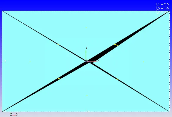
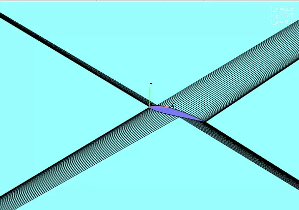
1. Use the coordinates provided in .DAT file for NACA 2412 Airfoil and create the airfoil using Geometry creation tools in converge.

2. Create points as per the .DAT file and join the dots by creating triangles and offset the geometry to create a 3D airfoil.

3. Create a wind tunnel having 3x from the inlet and 6x from the outlet and 2x top and bottom, where x is the chord length(airfoil length).

4. Join the tunnel vertices to the airfoil and delete the internal faces of the airfoil keeping it hollow for ecternal air flow simulations.

- Case setup:

1. Application type: time based

2. Materials:

a. Gas simulation: air

b. Global transport properties: Deafult

c. Species: O2 and N2

3. Simulation parameters:

a. Run parameters:

Transient solver, full hydrodynamic, compressible

b. Simulation time parameters:

- End time- 0.207 cycles

Calculating end time:

End time is calculated by analysing the flow time from the inlet to outlet and the inlet velocity at which the flow generates, by knowing these 2 parameters, we can calculate the end time.

Since, length of the domain is approx 2.5m and velocity at inlet = 36.196 m/s

Therefore, end time = distance of pipe/ inlet velocity

Which implies, 2.5/36.196= 0.0690 sec

It takes 0.0690 secs for the flow to complete 1 cycle, we can have 3 cycles which is 3x0.0690= 0.207 `~=`0.2secs

- Time step- 1e-6

- min time step- 1e-6

- max time step- 1

- Convection CFL number- 0.5

c. Solver Parameters-

- Solver type- density based solver

- Equations- pressure- change preconditioner to none

4. Boundary Conditions-

a. Inlet- Inflow

- Velocity inlet: 36.1969 m/s

- Initial temp- 300K

- Species boundary condition- add air

b. Wing- WALL

- Surface movement- FIXED

-Law of wall

- Turbulent kinetic energy(tke): NE

c. Outlet - outflow

-Pressure BC: NE (neuman BC)

- Backflow: DI, T= 300K, add airflow

d. Top and bottom wall: Wall

- Slip condition

- tke: DI

- Temperature BC: NE

e. Front and Back: 2D

- 2D wall

5. Initial Conditions and Events:-

- Regions and Initialization: Fluid flow region

Velocity: x= 36.1969 m/s

Pressure- 1e5 Pa

Temperature: 300K

Add- air

6. Physical Models:-

- RNG k-epsilon

7. Grid Control:-

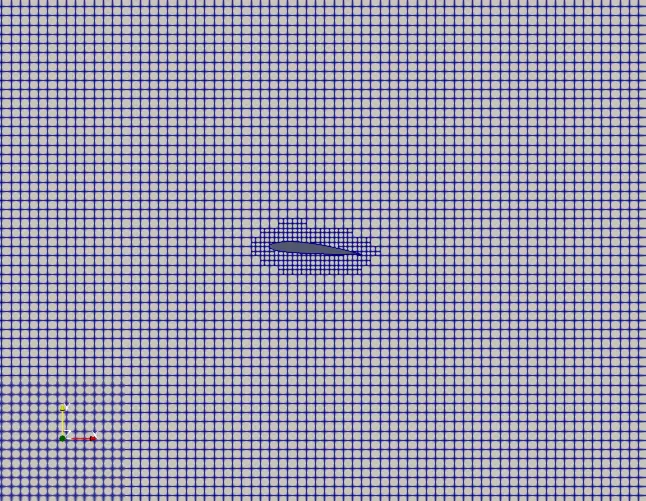
a. Base Grid:

dx = 0.01m, dy = 0.01m, dz = 0.01m

b. Embedding:

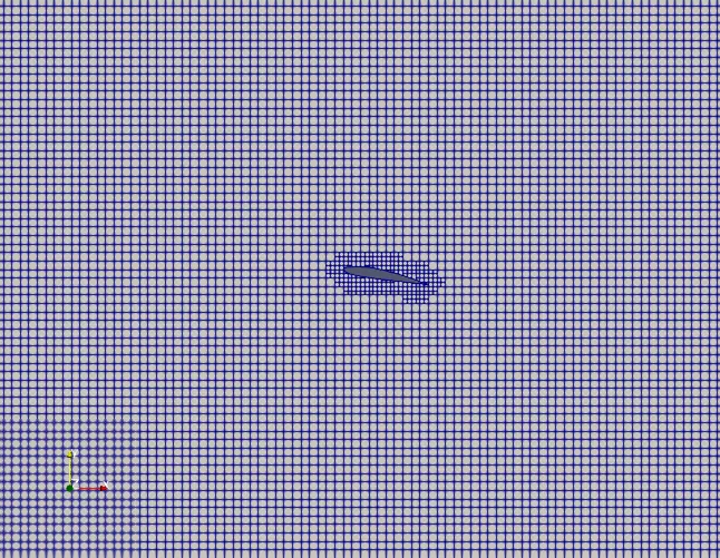
- Boundary type, Wing, permanent mode embedding.

Scale- 1

Number of layers- 3

Embedding is the means by which we can refine the mesh to a value that is lower than the prevalent base size. This is especially useful if we are looking to refine near wall to capture the boundary layer or the wake of a body more accurately.

8. Post-Processing:-

- Post Variable Selection:

Select the parameters needed to be post processed.

- Output files:

- output generation: wall output= Boundaries only ; this helps in retriving the pressure forces in X and Y direction which helps in figuring out the drag and lift forces

We need to set a time interval for the files to be saved during each set of iterations. It is best suited to have a min of 100 saved files for every simulation. Therefore we need to calculate the time interval for writing the output files based on our end time given in run parameters.

Restart files help in restoring the files if there is a sudden power cut/ crash which is not helpful or might end up loosing the entire data, therefore the restart files helps in resuming the simulation form the point we lost contact. Restart files time interval can be same as the writing files interval which is safe and healthy.

In this case- since the end time is 0.207, we can have a time interval of 0.1 and the total files created will be 100.

• Results:

- Mesh:

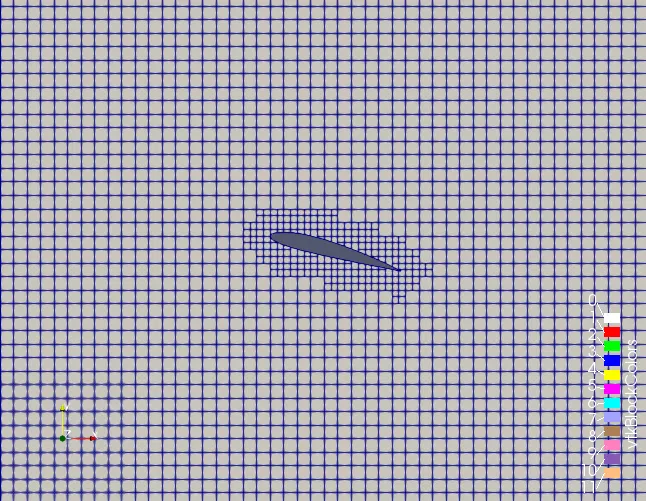
An Adaptive mesh refinment is used along the walls of the wing to give a better accuracy of the physics at the wing region. A Y+ of 50 is considered and the first cell thickness is calculated as 4.5e-04. These values can be used to calculate the grid scale for AMR.

Fixed Embedding = Base grid/ `2^n`

Where,

n is the grid scale

Base grid= 0.01m

Fixed embedding(first cell thickness)=4.5e-04

Therefore, n=1

- Mesh grid:

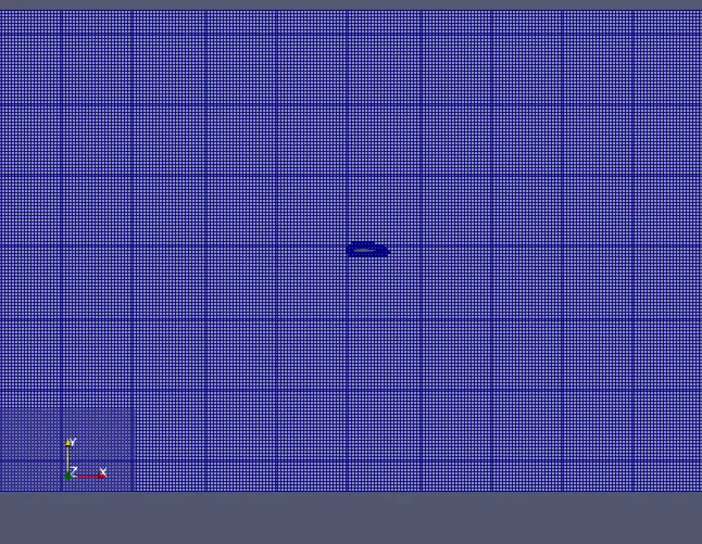
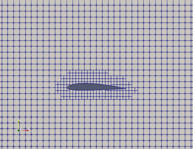
The challenge was carried using both steady and trasient state solver to analyse flow behaviour from both point of view. After carrying out steady state simulation, we found out that the simulation tends to blow up after a certain point where steady state solver lacks to calculate time averaging, therfore transient solver is preffered which is more accurate for external flow simulations.

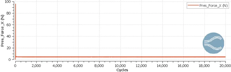
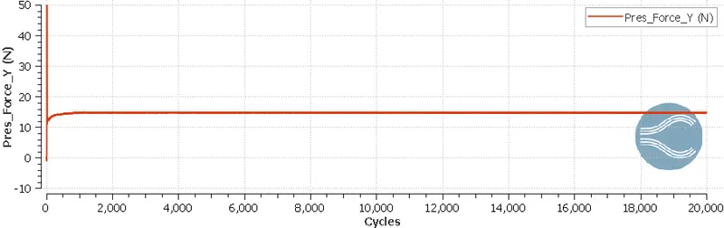
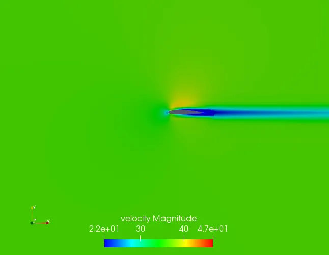
- Steady state simulation results (for 1 degree AOA):

1. Drag force:

2. Lift force:

3. Velocity contour:

4. Pressure contour:

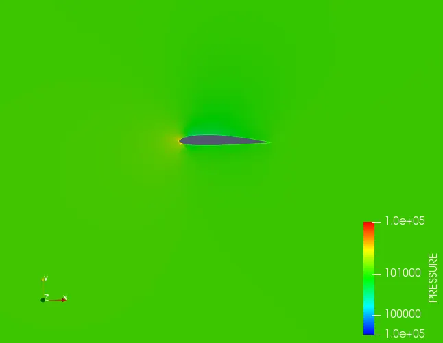
- Disscussion: It can be clearly viewed that the contours produced are incorrect and it doesnt do justice to the physics of the flow. The simulation tends to diverge and blow after certain number of iterations where the turbulence starts to increase and need for time averaging along the flow is necessary. Therefore, Transient state is used for furthur simulations.

- Transient State simulation:

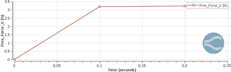
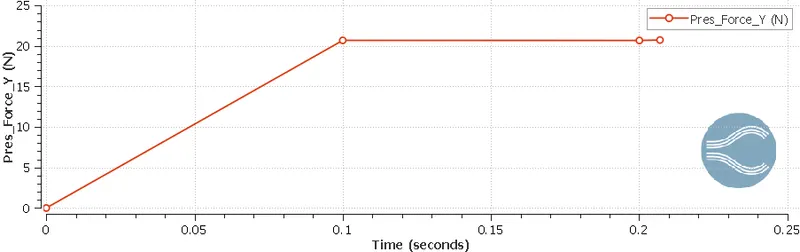
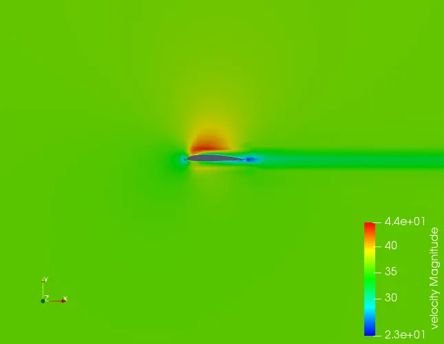
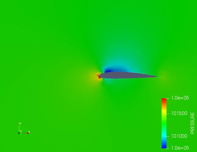
1. 1 Degree AOA:

a. Drag force:

b. Lift force:

c. Velocity contour:

d. Pressure contour:

2. 5 Degree AOA:

- Mesh:

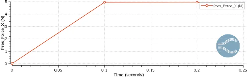
a. Drag force:

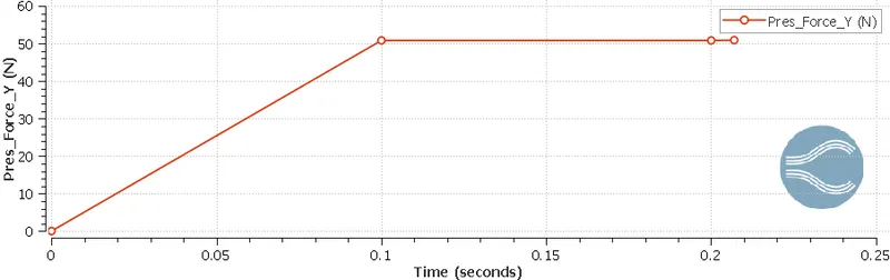
b. Lift force:

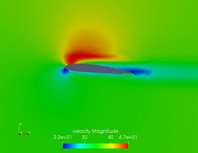
c. Velocity contour:

d. Pressure contour:

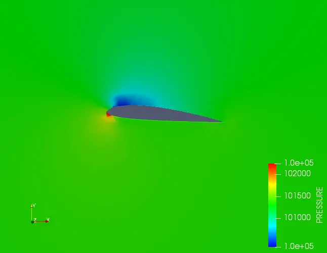
3. 10 Degree AOA:

- Mesh:

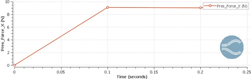
a. Drag force:

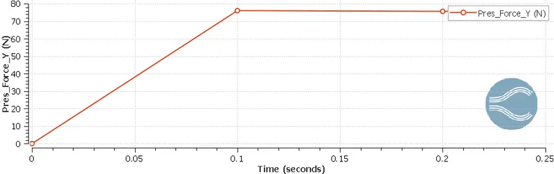
b. Lift force:

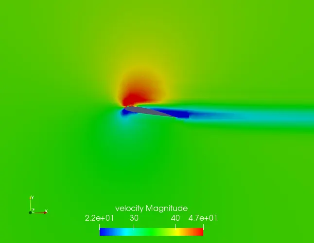
c. Velocity contour:

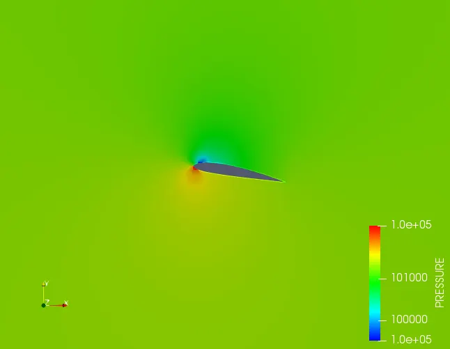
d. Pressure contour:

4. 15 Degree AOA:

- Mesh:

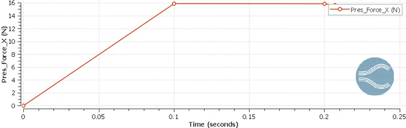
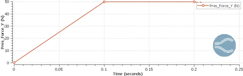
a. Drag force:

b. Lift force:

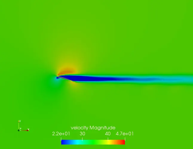
c. Velocity contour:

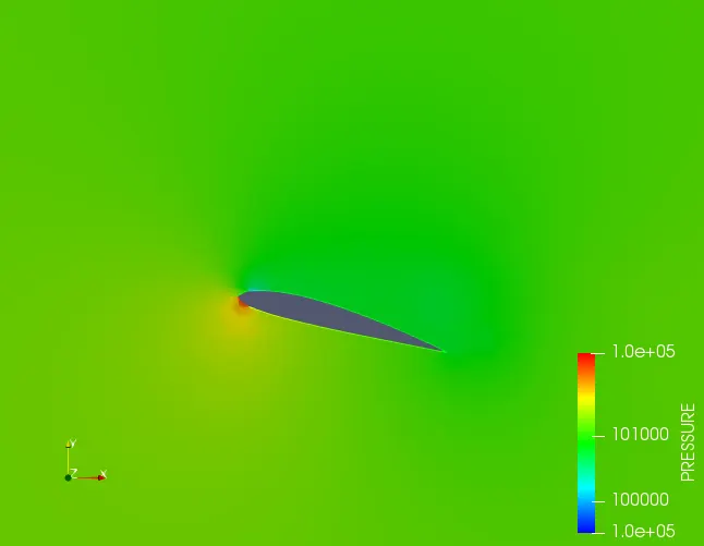
d. Pressure contour:

• Comparison of Coefficient of drag and lift with respect to angle of attack:

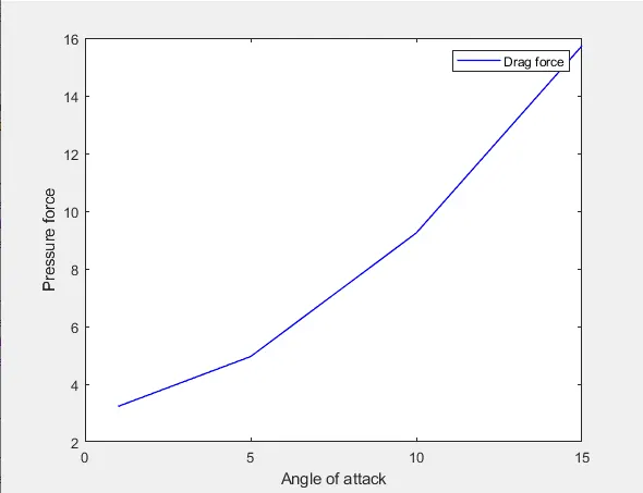
AOA	Drag force (Fd)	Lift force (Fl)	Coefficient of drag (Cd)	Coefficient of lift (Cl)
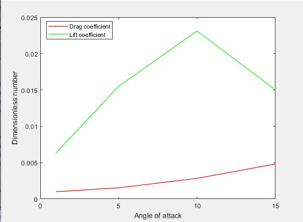
1	3.230	20.684	9.87e-04	0.00632
5	4.9590	50.921	1.52e-03	0.0155
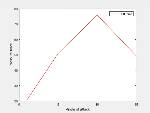
10	9.243	75.818	2.82e-03	0.0231
15	15.731	49.279	4.8e-03	0.0150

1. Drag force v/s Angle of attack:

2. Lift force v/s Angle of attack:

3. Coefficient of drag and lift v/s Angle of attack:

- Disscussions:

Transient state solver tends give better results than steady state since it uses time averaging method. The contours justify the physics and the plots explain the effect of drag and lift at different angle of attack. Drag increases as the frontal area increases and the lift increases until the flow undergoes flow seperation and then the lift reduces and undergoes stall.

• Conclusion:

1. The steady and transient simulation over an airfoil is achieved.

2. Use of Boundaries ly in the case setup helps in figuring the pressure forces acting in the X and Y direction which are drag and lift forces.

3. The graph clearly shows that as the angle of attack increases the drag increases, lift increases only until a optimum angle where the flow doesn't get separated.

4. But as the angles increases too much the flow tends to seperate and causes adverse pressure gradient which results in reverse flow and tends stall the aircraft and the lift reduces drastically. This tends to form vortices due to the turbulence produced and causes vibration.

5. Therefore it is optimal to use a AOA which gives a good lift below the stall angle.

6. Transient solver solves the problem more accurately than steady state solver, since transient solver solves the set of equations on each timestep on every cell which makes it more accurate and better time averaging.

7. In conclusion, While using Converge transient solver is preffered than the steady state for better accuracy and AMR is used for refinement at the wing region for accurate results.