Simulation of Simple pendulum using ODE in Matlab

1. Aim:

To write a Matlab program to solve 2^nd order ODE of a simple pendulum using the equation of motion of simple pendulum and to obtain the transient behaviour of the system.

2. Equations:

• Equation of motion of simple pendulum,

`(d^2 θ)/(dt^2 )+b/m dθ/dt+g/l sin⁡θ=0`

Where,

b = damping

m = mass

g = gravity

l = length

3. Objectives:

Write a program to solve the 2^nd order ODE of simple pendulum, to plot the transient movement of the pendulum and also use the data to simulate the change in displacement and velocity in the form of moving pendulum animation using the movie command.

4. Body of the content:

Programming language used: MATLAB

Before starting the program it is necessary to break the ODE of order 2 to 2 different equation which is simplified and easier to code.

1. Coding of program with the initial inputs of damping, mass, length, gravity and to enter the input conditions, time points.

Ode command is used to call the sub function used in a different program. The default syntax of ODE i.e, ode45(@(main input arguments) ode_func(the remaining conditions).

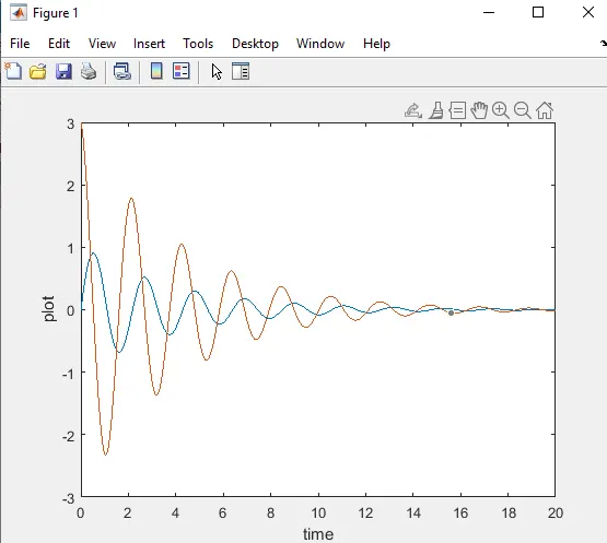
Using the plot command to obtain the transient behaviour of the motion by plotting the graph. The constant change in displacement and velocity can be depicted in the graph

1. Using the values obtained, a movie/animation can be achieved using the movie command, for loops is used to obtain the continuous motion of the pendulum.
2. Results/conclusion

This can be concluded and understood that with ODE can be solved using matlab by using the necessary commands and sub function. The needed animation can be created using the movie command and for loop.

Simulation/animation link: https://drive.google.com/file/d/16dRbT7Yccd6mg425geR7_Vd6hPjZ3M-z/view?usp=sharing

Main Program:

%program a 2 order ODE to plot and simulate the motion of simple pendulum
clear all
close all
clc
 
%input variables
b=0.05;
g=9.1;
l=1;
m=0.1;
 
%input conditions
theta_0=[0;3];
 
%time points (array)
t_span=linspace(0,20,500);
 
%to solve the ode using the default ode syntax
[t,results]=ode45(@(t,theta)ode_func(t,theta,b,g,l,m),t_span,theta_0);
 
%plotting of the graph
figure(1)
plot(t,results(:,1))
hold on 
plot(t,results(:,2))
ylabel('plot')
xlabel('time')
 
%creating the simulation 
ct=1;
for i=1:length(t_span)
    THETA1(i)=results(i,1);
    
    x0=0;
    y0=0;
    
    x1=1*sin(THETA1(i));
    y1=-1*cos(THETA1(i));
    
    figure(2)
    
    %base line for pendulum or support
    plot([-1 1],[0 0],'linewidth',4,'color','k')
    axis([-2 2 -1.5 0.5])
    hold on 
    
    %pendulum string 
    plot([x0 x1],[y0 y1],'linewidth',2,'color','r');
    hold on
    %pendulum ball
    plot(x1, y1,'.','markersize',50,'color','b')
    grid on
    hold off
    
    %using the movie command
    M(ct)=getframe(gcf)
    ct=ct+1;
end
 
%creating the movie clip
movie(M)
videofile=VideoWriter('Simple_pendulum.avi','uncompressed avi');
open(videofile)
writeVideo(videofile,M)
close(videofile)

Sub program(sub function):

function[dtheta_dt]= ode_func(t,theta,b,g,l,m)
 
%using the divided ode functions
theta1=theta(1)
theta2=theta(2)
dtheta1_dt=theta2;
dtheta2_dt=-(b/m)*theta2-(g/l)*sin(theta1);
dtheta_dt=[dtheta1_dt; dtheta2_dt];
end

Plot of the transient behaviour of motion of simple pendulum: