Mid term project - Solving the steady and unsteady 2D heat conduction problem

AIM:

To solve the 2D heat conduction equation at steady and transient state. Obtain convergence of by using explicit and implicit methods, and using iterative solvers to solve implicitly.

OBJECTIVE:

• Solve the 2D heat conduction equation by using explicit and implicit methods
• Solve the implicit method using point iterative techniques.
• The Boundary conditions for the problem are as follows;
• Top Boundary = 600 K
• Bottom Boundary = 900 K
• Left Boundary = 400 K
• Right Boundary = 800 K

• You will implement the following methods for solving implicit equations.

• Jacobi
• Gauss-seidel
• Successive over-relaxation

• Your absolute error criteria are 1e-4
• You will write code for both implicit and explicit schemes (This is for the Transient Analysis only)

THEORY:

1. Heat conduction equation:

The heat equation is a certain partial differential equation. Solutions of the heat equation are sometimes known as caloric functions. The theory of the heat equation was first developed by Joseph Fourier in 1822 for the purpose of modelling how a quantity such as heat diffuses through a given region. The heat equation is closely related to spectral geometry. In image analysis, the heat equation is sometimes used to resolve pixilation and to identify edges. Following Robert Richtmyer and John von Neumann's introduction of "artificial viscosity" methods, solutions of heat equations have been useful in the mathematical formulation of hydrodynamical shocks. Solutions of the heat equation have also been given much attention in the numerical analysis

3D heat conduction equation:

`(delT)/(delt) - alpha((del^2T)/(delx^2) + (del^2T)/(dely^2) + (del^2T)/(delz^2))=0`

Since we are only considering the 2-dimensional heat conduction equation, the equation breakdown into

`(delT)/(delt) - alpha((del^2T)/(delx^2) + (del^2T)/(dely^2) )=0`

There are 2 states at which the equation can be solved, they are

1. Steady-state 2.Transient/unsteady state

1. Steady-state analysis:

The steady-state heat equation is by definition not dependent on time. In other words, it is assumed conditions exist such that:

`(delT)/(delt) =0`

This condition depends on the time constant and the amount of time passed since boundary conditions have been imposed. Thus, the condition is fulfilled in situations in which the time equilibrium constant is fast enough that the more complex time-dependent heat equation can be approximated by the steady-state case. Equivalently, the steady-state condition exists for all cases in which enough time has passed that the thermal field u no longer evolves in time.

In the steady-state case, a spatial thermal gradient may (or may not) exist, but if it does, it does not change in time. This equation, therefore, describes the end result in all thermal problems in which a source is switched on (for example, an engine started in an automobile), and enough time has passed for all permanent temperature gradients to establish themselves in space, after which these spatial gradients no longer change in time (as again, with an automobile in which the engine has been running for long enough). The other (trivial) solution is for all spatial temperature gradients to disappear as well, in which case the temperature becomes uniform in space, as well.

The equation is much simpler and can help to understand better the physics of the materials without focusing on the dynamic of the heat transport process. It is widely used for simple engineering problems assuming there is an equilibrium of the temperature fields and heat transport, with time.

The 2D heat conduction equation at steady state is given as,

`(del^2T)/(delx^2) + (del^2T)/(dely^2) =0`

The above steady-state equation is discretised into an algebraic form so that it can be used for computation.

Central differencing schemes for 2nd order derivative is used to discretise the equation, which follows as:

`(T(i-1,j)- 2T(i,j)+ T(i+1,j))/(Δx^2) + ( T(i,j-1)- 2T(i,j)+ T(i,j+1))/(Δy^2) = 0`

After simplifying the above equation we obtain,

`T(i,j)= 1/k((T(i-1,j)+T(i+1,j))/ (Δx^2)) + 1/k((T(i,j-1)+T(i,j+1))/ (Δy^2)) …...... (1)`

Where,

`k= (2(Δx^2+ Δy^2))/(Δx^2 *Δy^2)`

Equation (1) can now be solved implicitly using the different iterative solvers.

2.Unsteady/Transient analysis:

We applied the finite difference method to steady problems by discretizing the problem in the space variables and solving for temperatures at discrete points called the nodes. The solution obtained is valid for any time since under steady conditions the temperature does not change with time. In transient problems, however, the temperatures change with time as well as position, and thus the finite difference solution of transient problems requires discretization in time in addition to discretization in space. For example, consider a hot metal object that is taken out of the oven at an initial temperature of Ti at time t=0 and is allowed to cool in ambient air. If a time step of Δt= 5 min is chosen, the determination of the temperature distribution in the metal piece after 3 hours requires the determination of the temperatures 3x(60/5)=36 times, or in 36-time steps. Therefore, the computation time of this problem will be 36 times that of a steady problem.

The 2D heat conduction equation at unsteady state is given as:

`(delT)/(delt) - alpha((del^2T)/(delx^2) + (del^2T)/(dely^2) )=0`

Using the time marching approach, the above equation can be solved explicitly and implicitly,

1. Solving the equation explicitly follows as,

`T(i,j)= Told(i,j)+ α*Δt((Told(i-1,j)-2Told(i,j)+ Told(i+1,j))/ (delx^2) + (Told(i,j-1)-2Told(i,j)+ Told(i,j+1))/ (dely^2))`

Equation (2) can be used to solve explicitly

2. Solving the equation implicitly follows as,

`T(i,j)= (1/(1+2k1+2k2))*(k1(T(i-1,j)+T(i+1,j))+ k2(T(i,j-1)+T(i,j+1))) ….... (3)`

Where,

`k1= (αΔt)/ (delx^2) , k2= (αΔt)/( dely^2)`

Equation (3) can be used to solve implicitly using different iterative solvers.

2. Convergence:

The standard convergence condition (for any iterative method) is when the spectral radius of the iteration matrix is less than 1:

`rho (D^{-1}(L+U))<1`

A sufficient (but not necessary) condition for the method to converge is that matrix A is strictly or irreducibly diagonally dominant. Strict row diagonal dominance means that for each row, the absolute value of the diagonal term is greater than the sum of absolute values of other terms

3. Iterative solvers:

In computational mathematics, an iterative method is a mathematical procedure that uses an initial value to generate a sequence of improving approximate solutions for a class of problems, in which the n-th approximation is derived from the previous ones. A specific implementation of an iterative method, including the termination criteria, is an algorithm of the iterative method. An iterative method is called convergent if the corresponding sequence converges for given initial approximations. Mathematically rigorous convergence analysis of an iterative method is usually performed; however, heuristic-based iterative methods are also common.

In contrast, direct methods attempt to solve the problem with a finite sequence of operations. In the absence of rounding errors, direct methods would deliver an exact solution (like solving a linear system of equations Ax=b by Gaussian elimination). Iterative methods are often the only choice for nonlinear equations. However, iterative methods are often useful even for linear problems involving many variables (sometimes of the order of millions), where direct methods would be prohibitively expensive (and in some cases impossible) even with the best available computing power.

1.Jacobi method:

In numerical linear algebra, the Jacobi method is an iterative algorithm for determining the solutions of a strictly diagonally dominant system of linear equations. Each diagonal element is solved for, and an approximate value is plugged in. The process is then iterated until it converges. This algorithm is a stripped-down version of the Jacobi transformation method of matrix diagonalization. The method is named after Carl Gustav Jacob Jacobi.

The matrix form is , X= TX + C

Where T is the iterative matrix and C is the constant and X is the temperature value changing at each node and time step.

2. Gauss-Seidel method:

In numerical linear algebra, the Gauss-Seidel method, also known as the Liebmann method or the method of successive displacement, is an iterative method used to solve a system of linear equations. It is named after the German mathematician's Carl Friedrich Gauss and Philipp Ludwig von Seidel, and is similar to the Jacobi method. Though it can be applied to any matrix with non-zero elements on the diagonals, convergence is only guaranteed if the matrix is either strictly diagonally dominant, or symmetric and positive definite.

The element-wise formula for the Gauss-Seidel method is extremely similar to that of the Jacobi method.

The computation of x(k+1) uses the elements of x(k+1) that have already been computed, and only the elements of x(k) that have not been computed in the k+1 iteration. This means that, unlike the Jacobi method, only one storage vector is required as elements can be overwritten as they are computed, which can be advantageous for very large problems.

However, unlike the Jacobi method, the computations for each element cannot be done in parallel. Furthermore, the values at each iteration are dependent on the order of the original equations.

Gauss-Seidel is the same as SOR (successive over-relaxation) with omega =1.

The convergence properties of the Gauss-Seidel method are dependent on the matrix A. Namely, the procedure is known to converge if either:

• A is symmetric positive-definite, or
• A is strictly or irreducibly diagonally dominant.

The Gauss-Seidel method sometimes converges even if these conditions are not satisfied.

3. Successive over-relaxation(SOR):

In numerical linear algebra, the method of successive over-relaxation (SOR) is a variant of the Gauss-Seidel method for solving a linear system of equations, resulting in faster convergence. A similar method can be used for any slowly converging iterative process.

It was devised simultaneously by David M. Young Jr. and by Stanley P. Frankel in 1950 for the purpose of automatically solving linear systems on digital computers. Over-relaxation methods had been used before the work of Young and Frankel. An example is the method of Lewis Fry Richardson and the methods developed by R. V. Southwell. However, these methods were designed for computation by human calculators, requiring some expertise to ensure convergence to the solution which made them inapplicable for programming on digital computers. These aspects are discussed in the thesis of David M. Young Jr.

The convergence rate for the SOR method can be analytically derived. One needs to assume the following

• the relaxation parameter is appropriate: omega belongs to (0,2)
• Jacobi's iteration matrix C{Jac}}:=I-D^{-1}A has only real eigenvalues
• Jacobi's method is convergent: `mu`:=rho (C_{Jac})<1
• a unique solution exists: |det A| not equal to 0

The method depends on the value of α where, α>1 is over relaxed and when α<1 is under relaxed.

PROGRAM:

1. Steady-state :

The steady-state equation is solved implicitly using Jacobi, Gauss-Siedel and SOR iterative techniques.

1. Jacobi (steady-state):

When the steady-state equation is numerically discretised using the central differencing scheme. we get,

`(T(i-1,j)- 2T(i,j)+ T(i+1,j))/(Δx^2) + ( T(i,j-1)- 2T(i,j)+ T(i,j+1))/(Δy^2) = 0`

After simplifying the above equation we obtain,

`T(i,j)= 1/k((T(i-1,j)+T(i+1,j))/ (Δx^2)) + 1/k((T(i,j-1)+T(i,j+1))/ (Δy^2))`

Where,

`k= (2(Δx^2+ Δy^2))/(Δx^2 *Δy^2)`

Therefore the function code used while solving for steady-state jacobi is,

function [T, jacobi_it]= jacobi(error,tol,T,nx,ny,l,b)

dx= l/(nx-1);
dy= b/(ny-1);

Told=T;

%initialing k value
k1= (dy^2)/(2*(dx^2+dy^2));
k2= (dx^2)/(2*(dx^2+dy^2));

%jacobi method
    jacobi_it= 1;
    while(error>tol)
        for i= 2:nx-1
            for j=2:ny-1
                T(i,j)=k1*(Told(i-1,j)+Told(i+1,j))+k2*(Told(i,j-1)+Told(i,j+1));
            end
        end
        error= max(max(abs(Told - T)));
        Told= T;
        jacobi_it = jacobi_it+1; 
    end

figure(1)
[a ,b]=contourf(T);
set(gca,'YDIR','reverse');
colorbar;
clabel(a,b);
xlabel('X-axis')
ylabel('Y-axis')
title_text2= sprintf('Iteration number= %d',jacobi_it);
title_text1=sprintf('Steady state (Jacobi)');
title(title_text1, title_text2)
end

ii. Gauss-Siedel (steady-state):

This method is very similar to that of Jacobi but only the values for the nodes which are already found are replaced with the old values for each iteration. This helps in solving the temperature equation more accurately with a lesser number of iterations

The function code for solving the equation using the Gauss-Siedel method is,

function [T, gs_it]= gauss_sidel(error,tol,T,nx,ny,l,b)

dx= l/(nx-1);
dy= b/(ny-1);

Told=T;

%initialing k value
k1= (dy^2)/(2*(dx^2+dy^2));
k2= (dx^2)/(2*(dx^2+dy^2));

% Gauss-sidel method
    gs_it= 1;
    while(error>tol)
        for i= 2:nx-1
            for j=2:ny-1
                T(i,j)=k1*(T(i-1,j)+Told(i+1,j))+k2*(T(i,j-1)+Told(i,j+1));
            end
        end
        error= max(max(abs(Told - T)));
        Told= T;
        gs_it = gs_it+1; 
    end

figure(2)
[a ,b]=contourf(T);
set(gca,'YDIR','reverse');
colorbar;
clabel(a,b);
xlabel('X-axis')
ylabel('Y-axis')
title_text2= sprintf('Iteration number= %d',gs_it);
title_text1=sprintf('Steady state (Gauss-sidel)');
title(title_text1, title_text2)
end

iii. Successive over-relaxation(SOR):

This method involves the use of either Gauss-seidel or Jacobi method, this method is an enhancer for Jacobi and gauss-seidel. This method helps in getting accurate answers and with the least number of iterations than Jacobi or gauss-seidel. This method involves the use of omega which is dependent on whether the terms are over-relaxed or under-relaxed.

The equation for the SOR method is:

T(i,j)= Told(i,j)(1-w) + w( T(gauss-siedel or jacobi)

The function code for solving the equation using the SOR method is,

function [T, sor_it]= sor(error,tol,T,nx,ny,l,b,w)

dx= l/(nx-1);
dy= b/(ny-1);

Told=T;

%initialing k value
k1= (dy^2)/(2*(dx^2+dy^2));
k2= (dx^2)/(2*(dx^2+dy^2));

% Sucessive over relaxation method
    sor_it= 1;
    while(error>tol)
        for i= 2:nx-1
            for j=2:ny-1
                T(i,j)=(1-w)*Told(i,j)+w*(k1*(T(i-1,j)+Told(i+1,j))+k2*(T(i,j-1)+Told(i,j+1)));
            end
        end
        error= max(max(abs(Told - T)));
        Told= T;
        sor_it = sor_it+1; 
    end

figure(3)
[a ,b]=contourf(T);
set(gca,'YDIR','reverse');
colorbar;
clabel(a,b);
xlabel('X-axis')
ylabel('Y-axis')
title_text2= sprintf('Iteration number= %d',sor_it);
title_text1=sprintf('Steady state (SOR)');
title(title_text1, title_text2)
end

2. Unsteady-state :

The 2D heat conduction eqution is,

`(delT)/(delt) - alpha((del^2T)/(delx^2) + (del^2T)/(dely^2) )=0`

Using the time marching approach, the above equation can be solved explicitly and implicitly,

1. Solving the equation explicitly follows as,

`T(i,j)= Told(i,j)+ α*Δt((Told(i-1,j)-2Told(i,j)+ Told(i+1,j))/ (delx^2) + (Told(i,j-1)-2Told(i,j)+ Told(i,j+1))/ (dely^2))`

Equation (2) can be used to solve explicitly

2. Solving the equation implicitly follows as,

`T(i,j)= (1/(1+2k1+2k2))*(k1(T(i-1,j)+T(i+1,j))+ k2(T(i,j-1)+T(i,j+1))) ….... (3)`

Where,

`k1= (αΔt)/ (delx^2) , k2= (αΔt)/( dely^2)`

i. Explicit method(unsteady):

Explicit method is much easier to solve and compute the values calculated at the current time steps using the previous time step values, but the solution accuracy is much than the implicit methods and the number of iterations needed to converge is much lesser than the implicit since there are no unknown values to compute.

the function code to solve the equation explicitly is,

function [T, explicit_it]= explicit(error,tol,T,nx,ny,l,b,a)

dx= l/(nx-1);
dy= b/(ny-1);

Told=T;

dt= 0.5/((a/dx^2)+(a/dy^2));
%initialing k value
k1= (a*dt)/(dx^2);
k2= (a*dt)/(dy^2);

%Unsteady explicit method
    explicit_it= 1;
    while(error>tol)
        for i= 2:nx-1
            for j=2:ny-1
                T(i,j)=Told(i,j)+k1*(Told(i-1,j)-2*(Told(i,j))+Told(i+1,j))+k2*(Told(i,j-1)-2*(Told(i,j))+Told(i,j+1));
            end
        end
        error= max(max(abs(Told - T)));
        Told= T;
        explicit_it = explicit_it+1; 
    end

figure(4)
[a ,b]=contourf(T);
set(gca,'YDIR','reverse');
colorbar;
clabel(a,b);
xlabel('X-axis')
ylabel('Y-axis')
title_text2= sprintf('Iteration number= %d',explicit_it);
title_text1=sprintf('Unsteady state (explicit)');
title(title_text1, title_text2)
end

ii. Implicit (unsteady)

a. Jacobi(unsteady):

Solving the unsteady equation implicitly using the Jacobi method is similar to that of steady-state Jacobi, but here since there is a time-dependent variable dt, therefore there is a need for time loop where the value is iterated for every time loop. and the previous time step values are in the current time step to calculate the temperature values for accurately.

The function code for unsteady Jacobi method is,

function [T_unsteady_jacobi, un_j_it]= un_jacobi(tol,T,nx,ny,l,b,a)

dx= l/(nx-1);
dy= b/(ny-1);

T_unsteady_jacobi=T;
Tprev=T;

dt= 0.5/((a/dx^2)+(a/dy^2));
%initialing k value
k1= (a*dt)/(dx^2);
k2= (a*dt)/(dy^2);

term1= (1+(2*k1)+(2*k2))^-1;
term2= k1*term1;
term3= k2*term1;
error1= 9e9;

%Unsteady jacobi method
 un_j_it= 1;
 time_step=1;
 while(error1>tol)
     error=9e9;
    while(error>tol)
        for i= 2:nx-1
            for j=2:ny-1
                T_unsteady_jacobi(i,j)=(term1*Tprev(i,j))+ (term2*(T(i-1,j)+T(i+1,j)))+ (term3*(T(i,j-1)+T(i,j+1)));
            end
        end
        error= max(max(abs(T - T_unsteady_jacobi)));
        T= T_unsteady_jacobi;
        un_j_it = un_j_it +1;
    end
    error1= max(max(abs(Tprev-T_unsteady_jacobi)));
    Tprev=T;
    time_step= time_step+1;
 end
figure(5)
[a ,b]=contourf(T);
set(gca,'YDIR','reverse');
colorbar;
clabel(a,b);
xlabel('X-axis')
ylabel('Y-axis')
title_text2= sprintf('Iteration number= %d',un_j_it);
title_text1=sprintf('Unsteady state (Jacobi)');
title(title_text1, title_text2)
end

b. Gauss-Seidel (unsteady):

This is similar to unsteady state Jacobi but only the T_old values change after each iteration in space loop till the error term becomes greater than the tolerance value.

The function code for unsteady-state Gauss-seidel is,

function [T_unsteady_gs, un_gs_it]= un_gs(tol,T,nx,ny,l,b,a)

dx= l/(nx-1);
dy= b/(ny-1);

T_unsteady_gs=T;
Tprev=T;

dt= 0.5/((a/dx^2)+(a/dy^2));
%initialing k value
k1= (a*dt)/(dx^2);
k2= (a*dt)/(dy^2);

term1= (1+(2*k1)+(2*k2))^-1;
term2= k1*term1;
term3= k2*term1;
error1= 9e9;

%Unsteady jacobi method
 un_gs_it= 1;
 time_step=1;
 while(error1>tol)
     error=9e9;
    while(error>tol)
        for i= 2:nx-1
            for j=2:ny-1
                T_unsteady_gs(i,j)=(term1*Tprev(i,j))+ (term2*(T_unsteady_gs(i-1,j)+T(i+1,j)))+ (term3*(T_unsteady_gs(i,j-1)+T(i,j+1)));
            end
        end
        error= max(max(abs(T - T_unsteady_gs)));
        T= T_unsteady_gs;
        un_gs_it = un_gs_it +1;
    end
    error1= max(max(abs(Tprev-T_unsteady_gs)));
    Tprev=T;
    time_step= time_step+1;
 end
figure(6)
[a ,b]=contourf(T);
set(gca,'YDIR','reverse');
colorbar;
clabel(a,b);
xlabel('X-axis')
ylabel('Y-axis')
title_text2= sprintf('Iteration number= %d',un_gs_it);
title_text1=sprintf('Unsteady state (Gauss-sidel)');
title(title_text1, title_text2)
end

c. Successive over-relaxation (unsteady):

SOR for the unsteady is similar to that of steady-state but only the time loop is added therefore another error for the time loop is used so that the Tprev value is changed after each iteration.

The function code for unsteady SOR is,

function [T_unsteady_gs, un_gs_it]= un_gs(tol,T,nx,ny,l,b,a)

dx= l/(nx-1);
dy= b/(ny-1);

T_unsteady_gs=T;
Tprev=T;

dt= 0.5/((a/dx^2)+(a/dy^2));
%initialing k value
k1= (a*dt)/(dx^2);
k2= (a*dt)/(dy^2);

term1= (1+(2*k1)+(2*k2))^-1;
term2= k1*term1;
term3= k2*term1;
error1= 9e9;

%Unsteady jacobi method
 un_gs_it= 1;
 time_step=1;
 while(error1>tol)
     error=9e9;
    while(error>tol)
        for i= 2:nx-1
            for j=2:ny-1
                T_unsteady_gs(i,j)=(term1*Tprev(i,j))+ (term2*(T_unsteady_gs(i-1,j)+T(i+1,j)))+ (term3*(T_unsteady_gs(i,j-1)+T(i,j+1)));
            end
        end
        error= max(max(abs(T - T_unsteady_gs)));
        T= T_unsteady_gs;
        un_gs_it = un_gs_it +1;
    end
    error1= max(max(abs(Tprev-T_unsteady_gs)));
    Tprev=T;
    time_step= time_step+1;
 end
figure(6)
[a ,b]=contourf(T);
set(gca,'YDIR','reverse');
colorbar;
clabel(a,b);
xlabel('X-axis')
ylabel('Y-axis')
title_text2= sprintf('Iteration number= %d',un_gs_it);
title_text1=sprintf('Unsteady state (Gauss-sidel)');
title(title_text1, title_text2)
end

3. Main program

%Solving 2D heat conduction equation (steady and transisent problem)
%Steady state heat conduction equation is solved using implicit method and different iterative methods

clear all 
close all
clc

%input variables 
l=1;
b=1;
nx=10;
ny=nx;
x= linspace(0,1,nx);
y= linspace(0,1,ny);
a=1.5;
w=1.2;
error= 9e9;
tol= 1e-4;

%temperature boundary conditions

T_t= 600;
T_b= 900;
T_l= 400;
T_r= 800;
T= 300*ones(nx,ny);

%calculating the boundary temperatures
T(2:ny-1,1)=T_l;
T(2:ny-1,nx)=T_r;
T(1,2:nx-1)=T_t;
T(ny, 2:nx-1)= T_b;

%calculating the corner boundary temperatures
T(1,1)= (T_l+ T_t)/2;
T(nx,ny)= (T_r+ T_b)/2;
T(ny,1)= (T_l+ T_b)/2;
T(1,nx)= (T_t+ T_r)/2;

iterative_solver= 1;
[X,Y]=meshgrid(x,y);

%Steady state heat conduction equation, d^2T/dx^2 + d^2T/dy^2;
[T_j, jacobi_it]= jacobi(error,tol,T,nx,ny,l,b);

[T_gs, gs_it]= gauss_sidel(error,tol,T,nx,ny,l,b);

[T_sor, sor_it]= sor(error,tol,T,nx,ny,l,b,w);

%Unsteady state heat conduction equation, dT/dt + a(d^2T/dx^2 + d^2T/dy^2)
% Explicit method
[T_ex, explicit_it]= explicit(error,tol,T,nx,ny,l,b,a);

%Implicit method
%Jacobi method
[T_un_j, un_j_it]= un_jacobi(tol,T,nx,ny,l,b,a);

%Gauss-sidel method
[T_un_gs, un_gs_it]= un_gs(tol,T,nx,ny,l,b,a);

%successive over relaxation
[T_un_sor, un_sor_it]= un_sor(tol,T,nx,ny,l,b,a,w);

code explanation:

1. the main program is coded with the inputs variables, initial conditions and boundary conditions.

2.The domain is created by inputting the number of nodes, since its a 2D we have initiate nodes in x and y direction and create a uniform domain. i.e. nx=ny (number of nodes).

3. The temperature at the corners are calculated using the average of the temperatures.

4. the functions for explicit and each iterative solvers is called and the necessary outputs are plotted accordingly.

PLOTS:

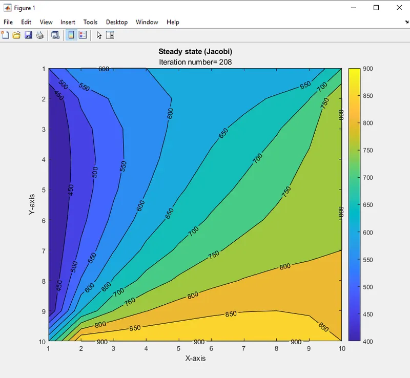
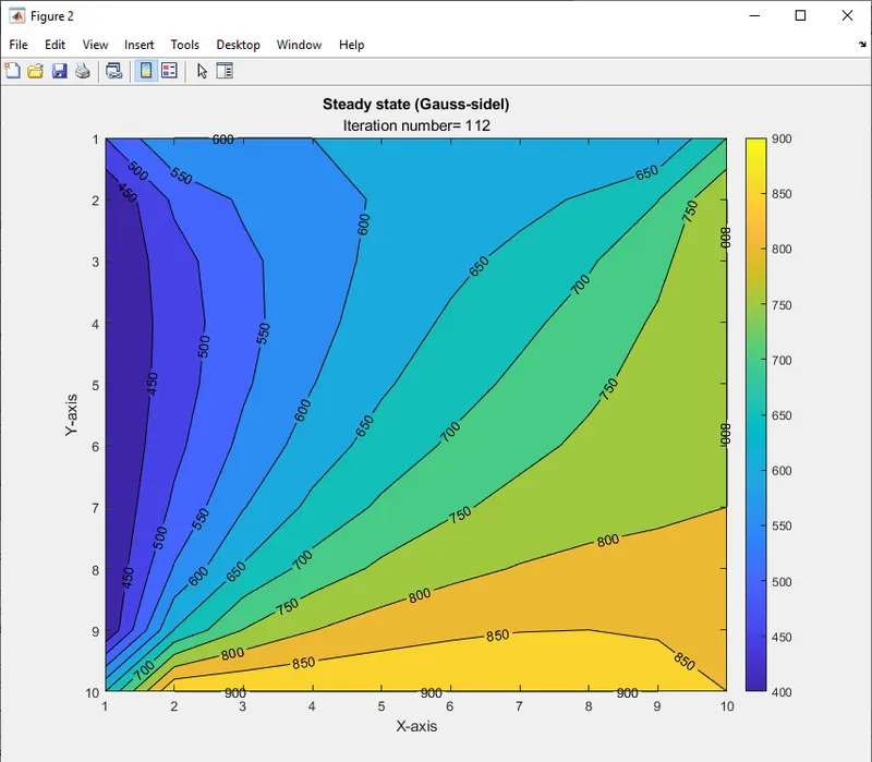
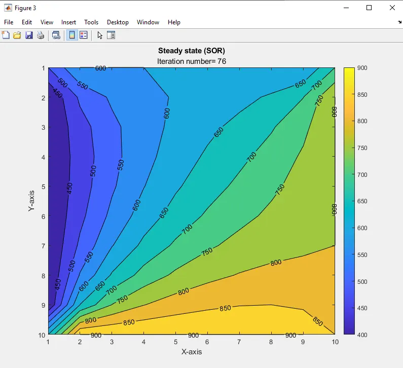
1. steady-state:

2. Unsteady state:

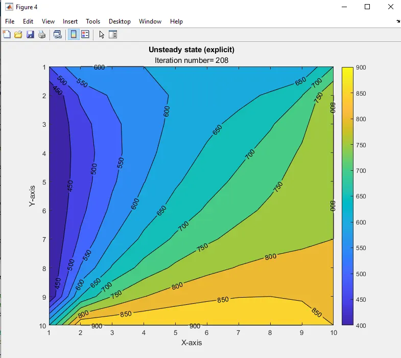
a. explicit:

b. Implicit:

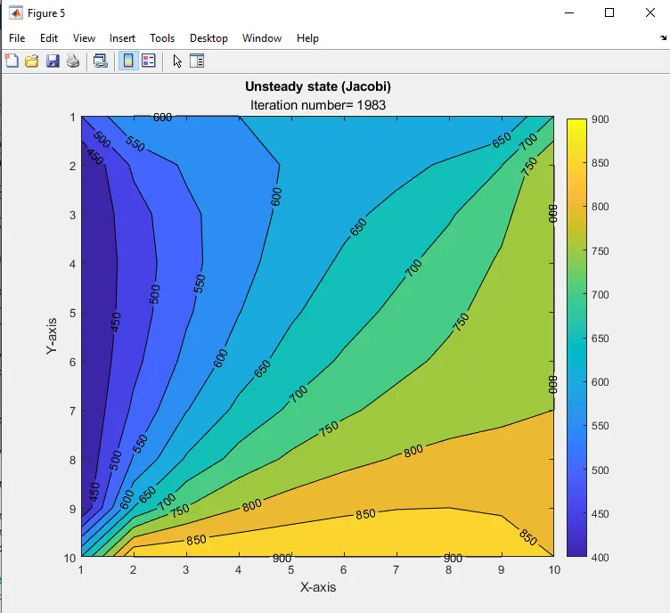
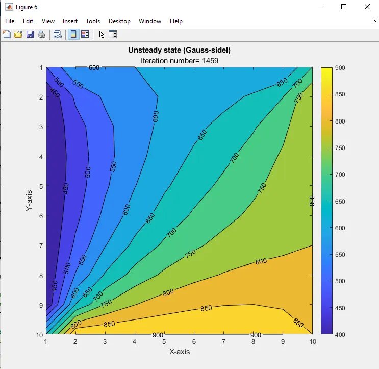
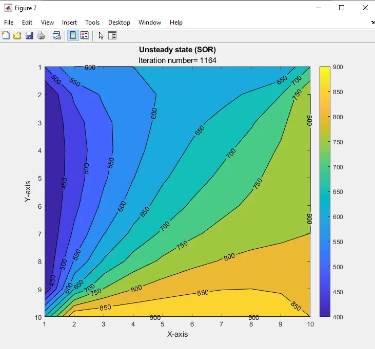
Results and Conclusion:

The number of iteration run by each method:

1. steady-state:

a. Jacobi : 208

b. Gauss-Seidel : 112

c. SOR : 76

2.Unsteady-state:

a. Explicit : 208

b. Jacobi : 1983

c. Gauss-Seidel : 1459

d. SOR : 1164

1. The successive over-relaxation method is much more effective than the other methods since the solution is converging at a much faster rate and lesser iterations than Jacobi and Gauss-Seidel methods. But the relaxation factor has to be kept in an ideal value so that if the value is high the solution might oscillate around the correct solution and if the factor is very less the solution might not converge.

2. It can be observed that explicit is much faster than the implicit methods and the simulation run time is also much lesser than implicit.

3. The number of iterations for steady-state is much lesser than the unsteady-state. That is because to change the unsteady state to steady-state we have to time march much longer than the steady-state therefore the iteration numbers are more.

4. The CFL number should be maintained less than 0.5 so that we can obtain converged results.

5. The implicit method is more accurate than the explicit method even though the number of iterations is much lesser since the implicit method uses all the points of the domain which makes it more accurate.