Rankine cycle Simulator
- Aim:
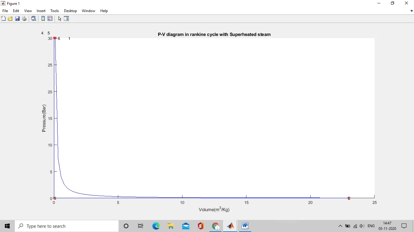
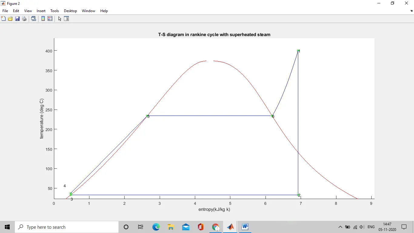
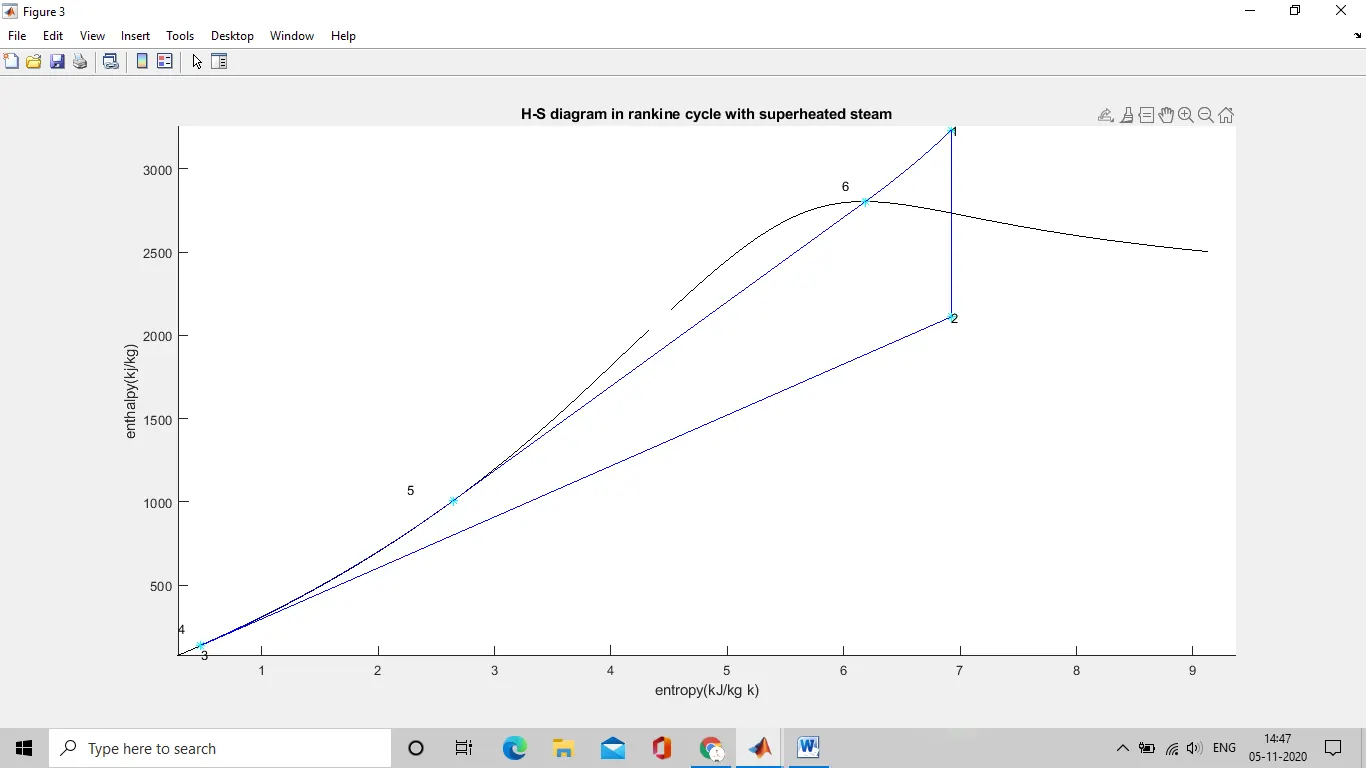
Calculating all the state points of a rankine cycle with the help of 3 inputs i.e, turbine inlet pressure, turbine inlet temperature and turbine outlet pressure. Deriving the outputs such as workdone by turbine, net workdone, thermal efficiency of the cycle, specific steam consumption are to be calculated and to be shown along with all state variables. Plots of P-V, T-S, H-S diagram is to be determined, all this has to be calculated and programmed using matlab.
- Objectives:
- To simulate rankine cycle using matlab.
- Plot T-S , H-S diagram of the cycle.
- calculate the state points of the cycle.
- Plot the graphs
- Code explanation.
Body of the content:
- Theory:
Rankine cycle:
The Rankine cycle is a model used to predict the performance of steam turbine systems. It was also used to study the performance of reciprocating steam engines. The Rankine cycle is an idealized thermodynamic cycle of a heat engine that converts heat into mechanical work while undergoing phase change. It is an idealized cycle in which friction losses in each of the four components are neglected. The heat is supplied externally to a closed loop, which usually uses water as the working fluid.
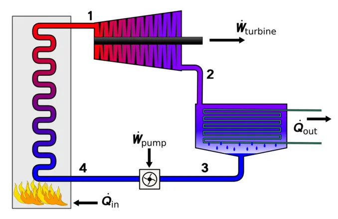
There are four processes in the Rankine cycle. The states are identified by numbers (in brown) in the T–s diagram.
- Process 1–2: The working fluid is pumped from low to high pressure. As the fluid is a liquid at this stage, the pump requires little input energy.
In other words Process 1-2 is [Isentropic compression]
- Process 2–3: The high-pressure liquid enters a boiler, where it is heated at constant pressure by an external heat source to become a dry saturated vapour. The input energy required can be easily calculated graphically, using an enthalpy–entropy chart, or numerically, using steam tables.
In other words Process 2-3 is [Constant pressure heat addition in boiler]
- Process 3–4: The dry saturated vapour expands through a turbine, generating power. This decreases the temperature and pressure of the vapour, and some condensation may occur. The output in this process can be easily calculated using the chart or tables noted above.
In other words Process 3-4 is [Isentropic expansion]
- Process 4–1: The wet vapour then enters a condenser, where it is condensed at a constant pressure to become a saturated liquid.
2.Coding explanation:
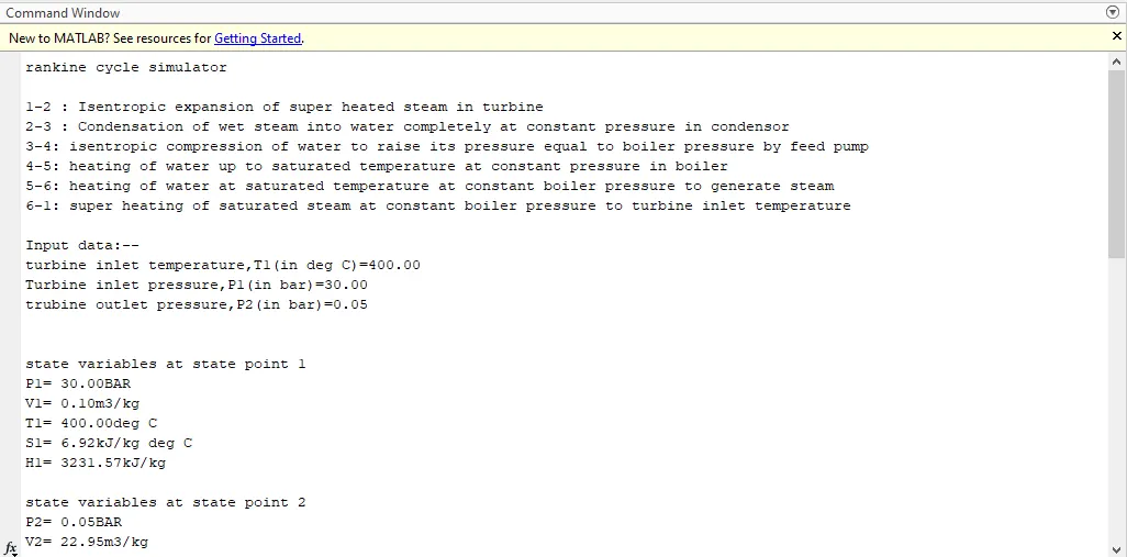
- Initially the input data is taken. These are turbine inlet pressure, P1=30Bar, Turbine inlet temperature, T1= 400 degC, Turbine outlet pressure, P2=0.05Bar.
- After that state variables for 6 state points, are calculated using the XSteam file is downloaded from the link given to get the steam table data.
- For the state point-1: T1,P1 are already given, value of V1(specific volume in m3/kg), H1(specific enthalpy in kJ/kg), S1(specific entropy in kJ/kg degC) are obtained from using the Xsteam library downloaded. Here we see the steam feed in to the turbine is superheated steam.
- Process 1-2 is isentropic expansion of steam in turbine. After expansion the steam becomes wet. Here entropy remains constant, S2=S1.
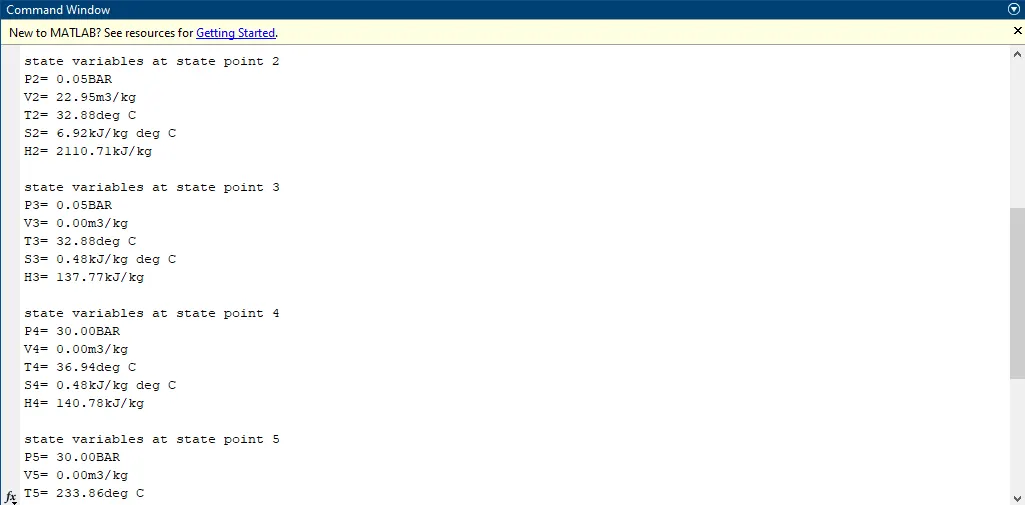
- So for the state point 2, the dryness fraction(x) of the steam is calculated. With the value of ‘x’ & by using XSteam library we get the values of S2, H2, V2 and T2 calculated. P2 is given as an input data.
- To get in between points of 1-2 process, the formula (pv^n=C) is used. Here the value of ‘n’ is calculated and from that, value of constant I evaluated. Hence the values of in between points of 1-2 process have been defined.
- Process 2-3, is a constant pressure and temperature process. Here wet steam from turbine is condensed in condenser into water completely.
- So for the state points 2 and 3, there are no change in pressure and temperature. So P2=P3 and T2=T3. Accordingly S3, H3 are calculated and V3 is obtained from XSteam library.
- The process 3-4 is isentropic compression of saturated water by feed pump. So here entropy remains constant (S3=S4). In the processes the pressure of water is raised to boiler pressure.
- Therefore, P4=P1 (P1 is boiler pressure). Here work is done by feed pump on water. Work done by feed pump is calculated, which is used to find out the enthalpy at state point 4 (H4=H3+wp).
- Cp4 & Cv4 ( specific heat of water at constant pressure and constant volume for state point 4) are calculated by using XSteam library. Cp4, Cv4 and formula (T^k*p^(k-1)=C, where k= cp4/cv4) are used to find the value of T4. V4 is calculated from XSteam library.
- The processes 4-5 is heating of water in boiler at constant boiler pressure (P4=P5=P1) and at the end of the process (at state point 5) it will be saturated water at pressure P1. The saturation temperature at pressure P1 is T5. For the state point 5, the values of V5, T5, H5, S5 are calculated using XSteam library.
- The processes 5-6 is the process of generating saturated dry steam. So heat given, is the latent heat to produce the dry saturated steam. So here pressure & temperature remain constant. So P6=P5=P1 (boiler pressure=40Bar), T6=T5. For the state point 6, V6, S6, H6 are calculated by using XSteam library.
- The process 6-1 is superheating the dry saturated steam at constant boiler pressure, to raise the temperature of steam to T1(turbine inlet temperature= 400degC which is one of the input data for this program). Here pressure remains constant so P6=P1 (which is also turbine inlet pressure).
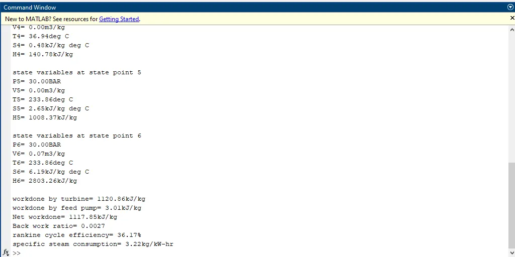
- After getting all the state variables, work done by turbine(w_t), work done by feed pump(wp), net work done(w_net), back work ratio(BWR), specific steam consumption (SSC) are calculated.
- After this the data to plot liquid line and dry saturated steam line is calculated. The critical temperature 374.15 degC is used here. At this critical point the latent heat of vaporization is 0 and at this point liquid and vapour phases merge and become identical in every respect. The corresponding pressure at this point is 221.2 bar.
- For getting points of liquid line and dry saturated line in T-S and H-S diagram, a for loop & XSteam library is used.
3.program:
% program to simulate and plot rankine cycle
clear all
close all
clc

%input data
%Turbine inlet pressure (in BAR)
p1=30;

%Turbine inlet temperature(in deg C)
t1=400;

%Turbine outlet pressure(in BAR)
p2=0.05;

%state variable at point 1,(turbine inlet point, super heated steam for
%boiler)
v1=XSteam('v_pT',p1,t1);
s1=XSteam('s_pT',p1,t1);
h1=XSteam('h_pT',p1,t1);

%state variables at point 2,(turbine outlet point)
t2=XSteam('Tsat_p',p2);
sg2=XSteam('sV_p',p2);
sf2=XSteam('sL_p',p2);
sfg2=sg2-sf2;
x=(s1-sf2)/sfg2;
s2=sf2+x*sfg2;

hf2=XSteam('hL_p',p2);
hg2=XSteam('hV_p',p2);
hfg2=hg2-hf2;
h2=hf2+x*hfg2;
vg2=XSteam('vV_p',p2);
v2=x*vg2;

%PV^n=constant, finding value of n
%p1*v1^n=p2*v2^n
n=(log(p2)-log(p1))/(log(v1)-log(v2));
c=p1*v1^n;
v_exp=linspace(v1,v2,100);
p_exp=c./(v_exp).^n;

%state variable at point 3
p3=p2;
t3=t2;
v3=XSteam('vL_p',p3);
hf3=hf2;
h3=hf3;
s3=sf2;

%state variable at point 4
p4=p1;
s4=s3;
%feed pump work
wp=v3*(p4-p3)*100;
%finding t4 using cp,cv
cp4=XSteam('Cp_ps',p4,s4);
cv4=XSteam('Cv_ps',p4,s4);
k=cp4/cv4;
t4=t3/((p3/p4)^((k-1)/k));

v4=XSteam('v_pt',p4,t4);
h4=h3+wp;

%state variable at point 5
p5=p1;
v5=XSteam('vL_p',p5);
t5=XSteam('Tsat_p',p5);
h5=XSteam('hL_p',p5);
s5=XSteam('sL_p',p5);

%state variable at point 6
p6=p1;
v6=XSteam('vV_p',p6);
t6=t5;
h6=XSteam('hV_p',p6);
s6=XSteam('sV_p',p6);

%workdone by turbine(w_t)
w_t=h1-h2;

%net workdone (w_net);
w_net=w_t-wp;

%back work ratio
bwr=wp/w_t;

%rankine cycle efficiency
e_r=(w_net/(h1-hf3-wp))*100;

%specific heat consumption (SSC);
SSC=3600/w_net;

%for getting data related to saturated water line & dry saturated steam
%line
t=linspace(1,374.15,1000);
for i=1:length(t)
    sl(i)=XSteam('sL_T',t(i)); %sl=entropy of saturated water
    sg(i)=XSteam('sV_T',t(i)); %sg=entropy of saturated steam
    hl(i)=XSteam('hL_T',t(i)); %hl=enthalpy of saturated water
    hg(i)=XSteam('hV_T',t(i)); %hg=enthalpy of saturated steam
end

%plotting p-v diagram
figure(1)
hold on
plot(v1,p1,'*','color','r')
text(v1+1,p1,'1');
plot(v_exp,p_exp,'color','b')
plot(v2,p2,'*','color','r')
text(v2,p2,'2');
plot([v2,v3],[p2,p3],'color','b')
plot(v3,p3,'*','color','r')
text(v3,p3,'3')
plot([v3,v4],[p3,p4],'color','b')
plot(v4,p4,'*','color','r')
text(v4-1,p4+1,'4')
plot([v4,v5],[p4,p5],'color','b')
plot(v5,p5,'*','color','r')
text(v5-0.5,p5+1,'5')
plot([v5,v6],[p5,p6],'color','b')
plot(v6,p6,'*','color','r')
text(v6+0.25,p6,'6')
plot([v6,v1],[p6,p1],'color','b')
xlabel('Volume(m^3/Kg)')
ylabel('Pressure(Bar)')
title('P-V diagram in rankine cycle with Superheated steam')

%plotting T-S diagram
figure(2)
hold on

%plotting liquid line in the T-S diagram
plot(sl,t,'color','r')

%plotting saturated steam line in T-S diagram
plot(sg,t,'color','r')

%plotting T-S diagram through state points
plot(s1,t1,'*','color','g')
text(s1,t1,'1')
plot([s1,s2],[t1,t2],'color','b')
plot(s2,t2,'*','color','g')
text(s2,t2,'2')
plot([s2,s3],[t2,t3],'color','b')
plot(s3,t3,'*','color','g')
text(s3,t3-10,'3')
plot([s3,s4],[t3,t4],'color','b')
plot(s4,t4,'*','color','g')
text(s4-0.2,t4+20,'4')
plot([s4,s5],[t4,t5],'color','b')
plot(s5,t5,'*','color','g')
text(s5,t5,'5')
plot([s5,s6],[t5,t6],'color','b')
plot(s6,t6,'*','color','g')
text(s6,t6,'6')

s61=linspace(s6,s1,1000);
for k=1:length(s61)
    t61(k)=XSteam('T_ps',p1,s61(k));
end
plot(s61,t61,'color','b')
xlabel('entropy(kJ/kg k)')
ylabel('temperature (deg C)')
title('T-S diagram in rankine cycle with superheated steam')

%plotting S-H diagram
figure(3);
hold on
plot(sl,hl,'color','k')
plot(sg,hg,'color','k')
plot(s1,h1,'*','color','c')
text(s1,h1,'1')
plot([s1,s2],[h1,h2],'color','b')
plot(s2,h2,'*','color','c')
text(s2,h2,'2')

h23=linspace(h2,h3,1000);
for q=1:length(h23)
    s23(q)=XSteam('s_ph',p2,h23(q));
end
plot(s23,h23,'color','b')
plot(s3,h3,'*','color','c')
text(s3,h3-50,'3')
plot([s3,s4],[h3,h4],'color','b')
plot(s4,h4,'*','color','c')
text(s4-0.2,h4+100,'4')

h45=linspace(h4,h5,500);
for m=1:length(h45)
    s45(m)=XSteam('s_ph',p1,h45(m));
end
plot(s45,h45,'color','b')
plot(s5,h5,'*','color','c')
text(s5-0.4,h5+70,'5')

s56=linspace(s5,s6,1000);
for r=1:length(s56)
    h56(r)=XSteam('h_ps',p1,s56(r));
end
plot(s56,h56,'color','b')
plot(s6,h6,'*','color','c')
text(s6-0.2,h6+100,'6')

h61=linspace(h6,h1,1000);
for n=1:length(h61)
    s61(n)=XSteam('s_ph',p1,h61(n));
end
plot(s61,h61,'color','b')
xlabel('entropy(kJ/kg k)')
ylabel('enthalpy(kj/kg)')
title('H-S diagram in rankine cycle with superheated steam')

%heading & process in the cycle.

fprintf('rankine cycle simulator');
fprintf('n');
fprintf('n');
fprintf('1-2 : Isentropic expansion of super heated steam in turbine');
fprintf('n');
fprintf('2-3 : Condensation of wet steam into water completely at constant pressure in condensor');
fprintf('n');
fprintf('3-4: isentropic compression of water to raise its pressure equal to boiler pressure by feed pump');
fprintf('n');
fprintf('4-5: heating of water up to saturated temperature at constant pressure in boiler');
fprintf('n');
fprintf('5-6: heating of water at saturated temperature at constant boiler pressure to generate steam');
fprintf('n');
fprintf('6-1: super heating of saturated steam at constant boiler pressure to turbine inlet temperature');
fprintf('n');
fprintf('n');

%input data
disp('Input data:--');
fprintf('turbine inlet temperature,T1(in deg C)=');
fprintf('%.2f',t1);
fprintf('n');
fprintf('Turbine inlet pressure,P1(in bar)=');
fprintf('%.2f',p1);
fprintf('n')
fprintf('trubine outlet pressure,P2(in bar)=');
fprintf('%.2f', p2);
fprintf('n')
fprintf('n')
fprintf('n')

%display of state variables of state point 1
fprintf('state variables at state point 1');
fprintf('n');
fprintf('P1= ');
fprintf('%.2f', p1);
fprintf('BAR');
fprintf('n');
fprintf('V1= ');
fprintf('%.2f',v1);
fprintf('m3/kg');
fprintf('n');
fprintf('T1= ');
fprintf('%.2f',t1);
fprintf('deg C');
fprintf('n');
fprintf('S1= ');
fprintf('%.2f',s1);
fprintf('kJ/kg deg C');
fprintf('n');
fprintf('H1= ');
fprintf('%.2f',h1);
fprintf('kJ/kg');
fprintf('n');
fprintf('n');

%display of state variables of state point 2
fprintf('state variables at state point 2');
fprintf('n');
fprintf('P2= ');
fprintf('%.2f', p2);
fprintf('BAR');
fprintf('n');
fprintf('V2= ');
fprintf('%.2f',v2);
fprintf('m3/kg');
fprintf('n');
fprintf('T2= ');
fprintf('%.2f',t2);
fprintf('deg C');
fprintf('n');
fprintf('S2= ');
fprintf('%.2f',s2);
fprintf('kJ/kg deg C');
fprintf('n');
fprintf('H2= ');
fprintf('%.2f',h2);
fprintf('kJ/kg');
fprintf('n');
fprintf('n');

%display of state variables of state point 3
fprintf('state variables at state point 3');
fprintf('n');
fprintf('P3= ');
fprintf('%.2f', p3);
fprintf('BAR');
fprintf('n');
fprintf('V3= ');
fprintf('%.2f',v3);
fprintf('m3/kg');
fprintf('n');
fprintf('T3= ');
fprintf('%.2f',t3);
fprintf('deg C');
fprintf('n');
fprintf('S3= ');
fprintf('%.2f',s3);
fprintf('kJ/kg deg C');
fprintf('n');
fprintf('H3= ');
fprintf('%.2f',h3);
fprintf('kJ/kg');
fprintf('n');
fprintf('n');

%display state variables of point 4
fprintf('state variables at state point 4');
fprintf('n');
fprintf('P4= ');
fprintf('%.2f', p4);
fprintf('BAR');
fprintf('n');
fprintf('V4= ');
fprintf('%.2f',v4);
fprintf('m3/kg');
fprintf('n');
fprintf('T4= ');
fprintf('%.2f',t4);
fprintf('deg C');
fprintf('n');
fprintf('S4= ');
fprintf('%.2f',s4);
fprintf('kJ/kg deg C');
fprintf('n');
fprintf('H4= ');
fprintf('%.2f',h4);
fprintf('kJ/kg');
fprintf('n');
fprintf('n');

%display state variables of point 5
fprintf('state variables at state point 5');
fprintf('n');
fprintf('P5= ');
fprintf('%.2f', p5);
fprintf('BAR');
fprintf('n');
fprintf('V5= ');
fprintf('%.2f',v5);
fprintf('m3/kg');
fprintf('n');
fprintf('T5= ');
fprintf('%.2f',t5);
fprintf('deg C');
fprintf('n');
fprintf('S5= ');
fprintf('%.2f',s5);
fprintf('kJ/kg deg C');
fprintf('n');
fprintf('H5= ');
fprintf('%.2f',h5);
fprintf('kJ/kg');
fprintf('n');
fprintf('n');

%display state variables of point 6
fprintf('state variables at state point 6');
fprintf('n');
fprintf('P6= ');
fprintf('%.2f', p6);
fprintf('BAR');
fprintf('n');
fprintf('V6= ');
fprintf('%.2f',v6);
fprintf('m3/kg');
fprintf('n');
fprintf('T6= ');
fprintf('%.2f',t6);
fprintf('deg C');
fprintf('n');
fprintf('S6= ');
fprintf('%.2f',s6);
fprintf('kJ/kg deg C');
fprintf('n');
fprintf('H6= ');
fprintf('%.2f',h6);
fprintf('kJ/kg');
fprintf('n');
fprintf('n');

%display of workdone by turbibe, workdone by pump, Net workdone,back work
%ratio, thermal efficiency, specific steam consumption
fprintf('workdone by turbine= ');
fprintf('%.2f',w_t);
fprintf('kJ/kg');
fprintf('n');

fprintf('workdone by feed pump= ');
fprintf('%.2f',wp);
fprintf('kJ/kg');
fprintf('n');

fprintf('Net workdone= ');
fprintf('%.2f',w_net);
fprintf('kJ/kg');
fprintf('n');

fprintf('Back work ratio= ');
fprintf('%.4f',bwr);
fprintf('n');

fprintf('rankine cycle efficiency= ');
fprintf('%.2f',e_r);
fprintf('%s','%');
fprintf('n');

fprintf('specific steam consumption= ');
fprintf('%.2f',SSC);
fprintf('kg/kW-hr');
fprintf('n');
4.Plots:
- P-V diagram of rankine cycle
2.T-S diagram of rankine cycle:
3. H-S diagram of rankine cycle:
- Results/conclusion
The required simulation of rankine cycle is achieved and the necessary plots are derived. All the state variables are calculated. These are then later used to calculate the different properties stated below in the command window.
Reference:
2. https://drive.google.com/file/d/1RK_fvrOj38CIaQvmLT1S3daqHnxKCGU-/view