Week 9 - Mini project - Flow over an Airfoil
Aim
- To simulate flow over airfoil
- Extract Lift force and Drag force
- Plot Coefficient of drag Vs angle of attack
- Plot coefficient of lift vs angle of attack
- Compare two turbulance models from the above results
Airfoil
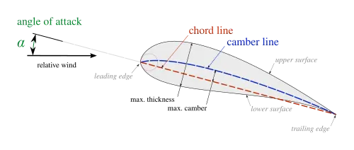
A solid body moving through a fluid produces an aerodynamic force. The component of this force perpendicular to the relative freestream velocity is called lift. The component parallel to the relative freestream velocity is called drag. An airfoil is a streamlined shape that is capable of generating significantly more lift than drag.[1] Airfoils designed for use at different speeds differ in their geometry: those for subsonic flight generally have a rounded leading edge, while those designed for supersonic flight tend to be slimmer with a sharp leading edge. All have a sharp trailing edge. Foils of similar function designed with water as the working fluid are called hydrofoils.
The lift on an airfoil is primarily the result of its angle of attack. When oriented at a suitable angle, the airfoil deflects the oncoming air (for fixed-wing aircraft, a downward force), resulting in a force on the airfoil in the direction opposite to the deflection. This force is known as aerodynamic force and can be resolved into two components: lift and drag. Most foil shapes require a positive angle of attack to generate lift, but cambered airfoils can generate lift at zero angle of attack. This "turning" of the air in the vicinity of the airfoil creates curved streamlines, resulting in lower pressure on one side and higher pressure on the other. This pressure difference is accompanied by a velocity difference, via Bernoulli's principle, so the resulting flowfield about the airfoil has a higher average velocity on the upper surface than on the lower surface. In some situations (e.g. inviscid potential flow) the lift force can be related directly to the average top/bottom velocity difference without computing the pressure by using the concept of circulation and the Kutta–Joukowski theorem.
Drag coefficient
In fluid dynamics, the drag coefficient (commonly denoted as  ,
,  or
or  is a dimensionless quantity that is used to quantify the drag or resistance of an object in a fluid environment, such as air or water. It is used in the drag equation in which a lower drag coefficient indicates the object will have less aerodynamic or hydrodynamic drag. The drag coefficient is always associated with a particular surface area.
The drag coefficient of any object comprises the effects of the two basic contributors to fluid dynamics drag: skin friction and form drag. The drag coefficient of a lifting airfoil or hydrofoil also includes the effects of lift-induced drag.The drag coefficient of a complete structure such as an aircraft also includes the effects of interference drag

 is the drag force,
  is the mass density of the fluid
 is the flow speed of the object relative to the fluid
 is the reference area
Lift coeffiecient
A fluid flowing around the surface of an object exerts a force on it. Lift is the component of this force that is perpendicular to the oncoming flow direction.It contrasts with the drag force, which is the component of the force parallel to the flow direction. Lift conventionally acts in an upward direction in order to counter the force of gravity, but it can act in any direction at right angles to the flow.
If the surrounding fluid is air, the force is called an aerodynamic force. In water or any other liquid, it is called a hydrodynamic force.
The lift coefficient (CL) is a dimensionless coefficient that relates the lift generated by a lifting body to the fluid density around the body, the fluid velocity and an associated reference area. A lifting body is a foil or a complete foil-bearing body such as a fixed wing aircraft. CL is a function of the angle of the body to the flow, its Reynolds number and its Mach number. The section lift coefficient cl refers to the dynamic lift characteristics of a two-dimensional foil section, with the reference area replaced by the foil chord
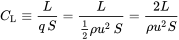
where  is the lift force,
 is the relevant surface area and
 is the fluid dynamic pressure, in turn linked to the fluid density
  , and to the flow speed
  .
.
Geometry
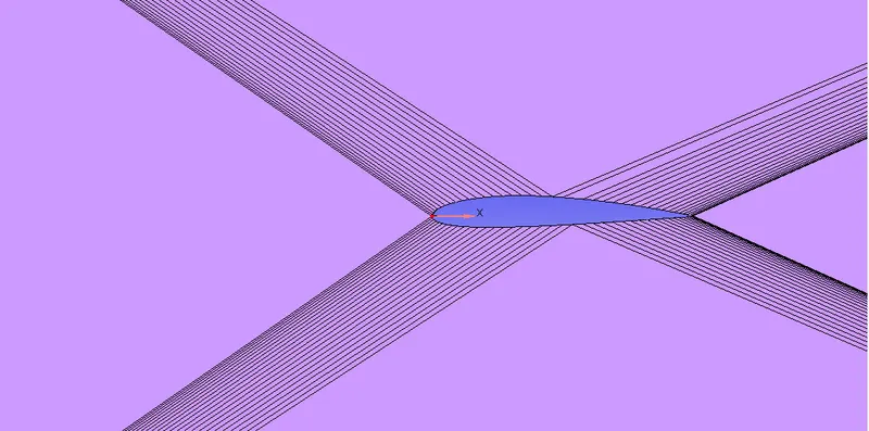
- The geometry is made by defining the co-ordinates for the vertices, the co-ordinates were taken from the co-ordinates of NACA 2412 airfoil
- It is then patched through selected vertices
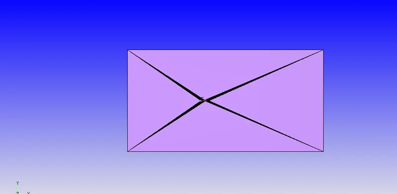
- Then a wind tunnel is made in rectangular shape
- Then it is patched followed by deletion of triangles inside the airfoil
- The whole geometry is copied to offset in z-direction by giving a value -1
- Now both the geometries are connected with triangles
Setup
- Calculation of inlet velocity
Re = 200000;
Mu = 0.000017894;
rho = 1.225;
D = 0.1
V = Re*Mu/(rho*D)
V = 29.2147 m/s
- Calculation of end time
Size of domain in flow direction = 2.4
Velocity at inlet = 29.2147 m/s
hence to complete a flow we would need at 2.4/29.2147 = 0.08 seconds to complete the flow through the given domain, however the end time is set to 0.4 seconds making the flow to happen multiple times
- In run parametres the minimum time step and initial time step is set to 1e-9 while the maximum time step is set to 1
- Transient simulation is set
- Boundary conditions are shown in screen shots
- In regions and initialisation a new region is created and gave it a velocity of 29.2147 m/s in x-direction
- For turbulence model our objective is to use both K-epsilon model and K-omega SST to check their differences in solutions
- Base grid is set to 0.04 m and the fixed embedding is selected as box type that covers an area where the more physics is expected it happen
- In output files the wall output is set to Boundaries only so that we can extract the lift and drag forces on airfoil wall
Outputs
K-Epsilon model
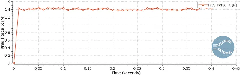
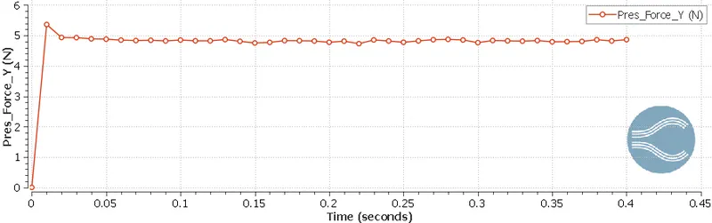
- Case 1 : 1 Degree angle of attack
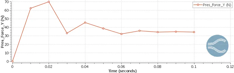
Drag force
Lift force
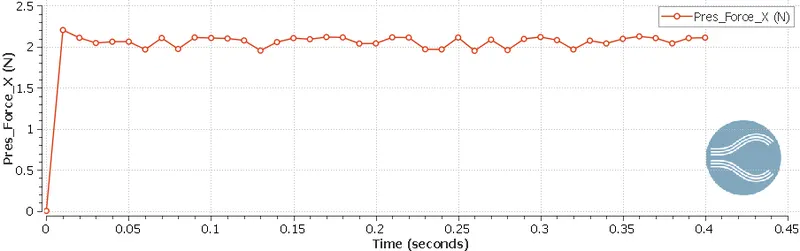
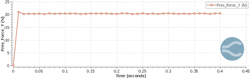
- Case 2 : 5 Degree angle of attack
Drag force
Lift force
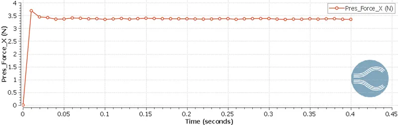
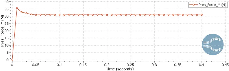
- Case 3 : 10 Degree angle of attack
Drag force
Lift force
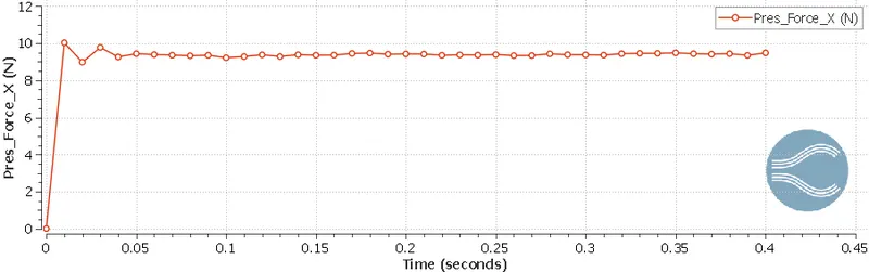
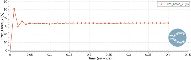
- Case 4 : 15 Degree angle of attack
Drag force
Lift force
Yplus
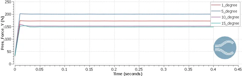
K-omega SST Model
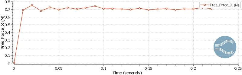
- Case 1 : 1 Degree angle of attack
Drag force
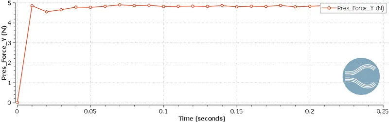
Lift force
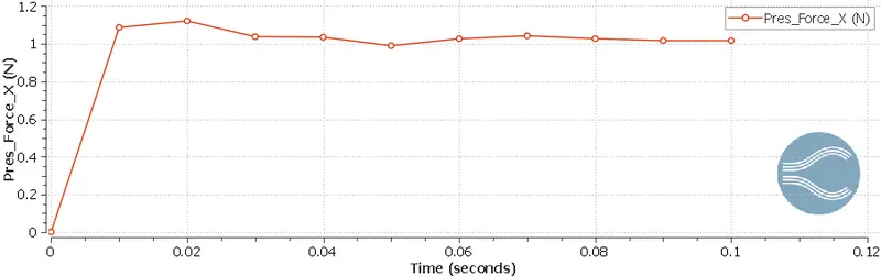
- Case 2 : 5 Degree angle of attack
Drag force
Lift force
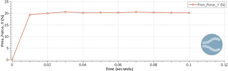
- Case 3 : 10 Degree angle of attack
Drag force
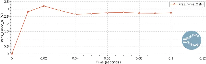
Lift force
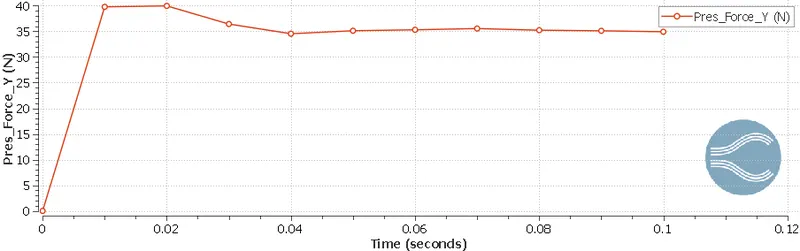
- Case 4 : 15 Degree angle of attack
Drag force
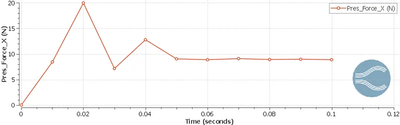
Lift force
Yplus
Calculations
Turbulance model : K-epsilon
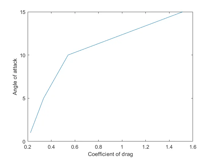
Drag coefficient
close all
clear all
clc

rho = 1.225  %density
A = 0.012    %reference area(max thickness of chord)
u = 29.2147  %Flow velocity
Fd_1 = 1.4   %Drag force for case 1
Fd_2 = 2.1   %Drag force for case 2
Fd_3 = 3.4   %Drag force for case 3
Fd_4 = 9.5   %Drag force for case 4
Cd_1 = 2*Fd_1/(rho*A*u^2)   %Drag coefficient for case 1
Cd_2 = 2*Fd_2/(rho*A*u^2)   %Drag coefficient for case 2
Cd_3 = 2*Fd_3/(rho*A*u^2)   %Drag coefficient for case 3
Cd_4 = 2*Fd_4/(rho*A*u^2)   %Drag coefficient for case 4

Alpha = [1 5 10 15];        %angle of attack
Cd = [Cd_1 Cd_2 Cd_3 Cd_4];

figure(1)
plot(Cd,Alpha)
xlabel('Coefficient of drag');
ylabel('Angle of attack')
Cd_1 = 0.2232
Cd_2 = 0.3348
Cd_3 = 0.542
Cd_4 = 1.5144
Coefficient of lift
close all
clear all
clc

rho = 1.225  %density
S = 0.1    %reference surface area(chord length)
u = 29.2147  %Flow velocity
L_1 = 5    %Lift force for case 1
L_2 = 20   %Lift force for case 2
L_3 = 30   %Lift force for case 3
L_4 = 34   %Lift force for case 4
Cl_1 = 2*L_1/(rho*S*u^2)   %Lift coefficient for case 1
Cl_2 = 2*L_2/(rho*S*u^2)   %Lift coefficient for case 2
Cl_3 = 2*L_3/(rho*S*u^2)   %Lift coefficient for case 3
Cl_4 = 2*L_4/(rho*S*u^2)   %Lift coefficient for case 4

Alpha = [1 5 10 15];        %angle of attack
Cl = [Cl_1 Cl_2 Cl_3 Cl_4];

figure(1)
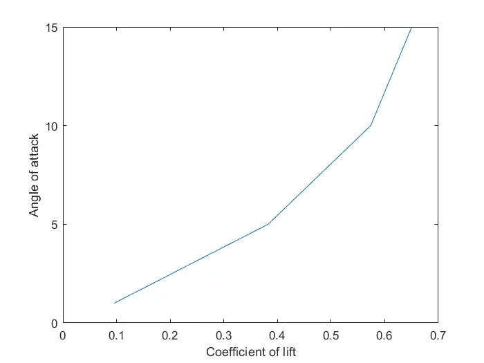
plot(Cl,Alpha)
xlabel('Coefficient of lift');
ylabel('Angle of attack')
Cl_1 = 0.0956
Cl_2 = 0.3826
Cl_3 = 0.5739
Cl_4 = 0.6504
Turbulance model : K-w SST
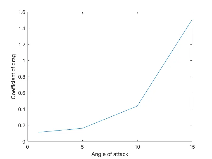
Drag coefficient
close all
clear all
clc

rho = 1.225                 %density
A = 0.012                   %reference area(chord thickness)
u = 29.2147                 %Flow velocity
Fd_1 = 0.708                %Drag force for case 1
Fd_2 = 1.01654              %Drag force for case 2
Fd_3 = 2.73706              %Drag force for case 3
Fd_4 = 9.4246               %Drag force for case 4
Cd_1 = 2*Fd_1/(rho*A*u^2)   %Drag coefficient for case 1
Cd_2 = 2*Fd_2/(rho*A*u^2)   %Drag coefficient for case 2
Cd_3 = 2*Fd_3/(rho*A*u^2)   %Drag coefficient for case 3
Cd_4 = 2*Fd_4/(rho*A*u^2)   %Drag coefficient for case 4

Alpha = [1 5 10 15];        %angle of attack
Cd = [Cd_1 Cd_2 Cd_3 Cd_4];

figure(1)
plot(Alpha,Cd)
xlabel('Angle of attack');
ylabel('Coefficient of drag')
Cd_1 = 0.1129
Cd_2 = 0.162
Cd_3 = 0.4363
Cd_4 = 1.5024
Lift Coefficient
close all
clear all
clc

rho = 1.225  %density
S = 0.1    %reference surface area(chord length)
u = 29.2147  %Flow velocity
L_1 = 4.84   %Lift force for case 1
L_2 = 20.1552   %Lift force for case 2
L_3 = 34.9485   %Lift force for case 3
L_4 = 33.4367  %Lift force for case 4
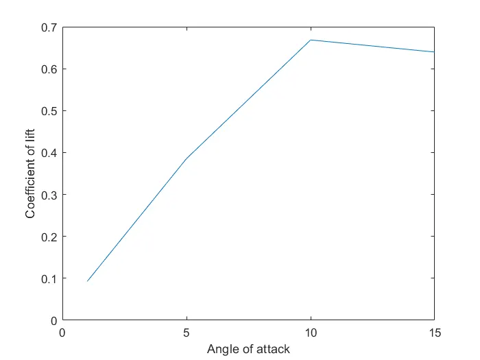
Cl_1 = 2*L_1/(rho*S*u^2)   %Lift coefficient for case 1
Cl_2 = 2*L_2/(rho*S*u^2)   %Lift coefficient for case 2
Cl_3 = 2*L_3/(rho*S*u^2)   %Lift coefficient for case 3
Cl_4 = 2*L_4/(rho*S*u^2)   %Lift coefficient for case 4

Alpha = [1 5 10 15];        %angle of attack
Cl = [Cl_1 Cl_2 Cl_3 Cl_4];

figure(1)
plot(Alpha,Cl)
xlabel('Angle of attack');
ylabel('Coefficient of lift')
Cl_1 = 0.0926
Cl_1 = 0.3855
Cl_1 = 0.6685
Cl_1 = 0.6396
Observations
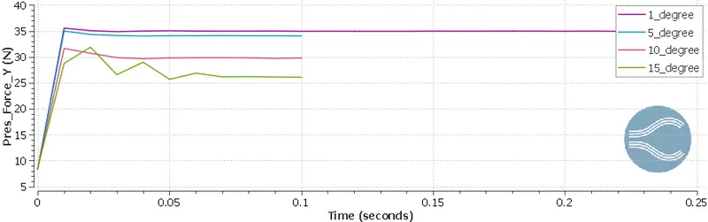
- The values in both turbulance model differ from each other, by looking at the y plus plots we can say that the yplus plot from k-epsilon turbulance model suggest that we are in the log-law region
- In order to capture the effects more precisely we need to be in viscous sublayer which has lower values of y-plus. Hence We can stick on to K-omega turbulance model for better results.
- The above theory can be confirmed by looking at the Coefficient of lift vs Angle of attack plot. Here after 10_degrees of angle of attack the lift drops. In actual we expect this phenomenon since the frontal area increases as a result of increased angle of attack the drag dominates and the adverse pressure gradients from the back of the wing causes stall
- K-omega SST turbulance model is well known for its uses in viscous sub-layer
- In velocity contour animations we can see that the flow over the air foil is less disruptive at lower level of angle of attack. At the 15 degree angle vortex shedding is formed which is very bad for airplanes to encounter
Conclusions
- Plotted Cd vs Angle of attack
- Plotted Cl vs Angle of attack
- Two types of turbulance models were compared and discussed
- Velocity contours were extracted