Week 7 - Simulation of a 1D Super-sonic nozzle flow simulation using Macormack Method
Subsonic-supersonic Nozzle
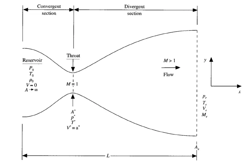
The flow at inlet to the nozzle comes from a reservoir where the pressure and temperature are denoted by `p_0` and `T_0` respectively. The cross-sectional area of the reservoir is large (thearotically A tends to infinity) and hence the velocity is very small and is value near to zero. Thus `p_0`and `T_0` are the stagnatuin values . The flow expands isentropically to supersonic speeds at the nozzle exit, where the exit pressure , temperature , velocity, and mach number are denoted by `p_e,T_e,v_e and M_e` respectively. The flow is locally subsonic in the convergent section of the nozzle, sonic at the throat (minimum rea), and supersonic at the divergent section. The sonic flow (m=1) at the throat means that the local velocity at this location is equal to the local speed of sound. Using an asterisk to denote sonic flow values, we have at the throat v = v* = a* . similarly the sonic flow values of pressure and temperature are denoted by p* and T*, respectively. The area of the sonic throat is denoted by *. Here we make an assumption that the flow varies only with x . that is flow properties are uniform at a given section. Such a flow is called Quasi-one -dimensional flow
Maccormack's technique
is an explicit finite difference technique which is second-order-accurate in both spce and time. This technique is student frendly and are perfectly satisfactory for many fluid applications. it follows three steges of calculations and they are
- Predictor step
Here we use Forward differencing for the space term
- Corrector step
Backward differencing is used here for the space terms
- Average step
This is simply the avarage of predictor and corrector step
these will be further clarified for each form
The governing equations for a non-conservative form
Continuity equation
`(delrho')/(delt') = -rho'*(delV')/(delx') - rho'V'(del(lnA'))/(delx') - V'(delrho')/(delx')`
Momentum equation
`(delV')/(delt') = -V'*(delV')/(delx') - (1)/(gamma)* ((delT')/(delx') + (T')/(rho')*(delrho')/(delx'))`
Energy equation
`(delT')/(delt') = -V'* (delT')/(delx') - (gamma-1)*T'((delV')/(delx') + V'*(del(lnA'))/(delx'))`
- Predictor step for the above formed equations
Continuity equation
`((delrho)/(delt))_(i)^N = -rho_i^N*(V_(i+1)^(N) - V_(i)^(N))/(trianglex) - rho_(i)^NV_(i)^N*(lnA_(i+1) - lnA_(i))/(trianglex) - V_(i)^*(rho_(i+1)^N - rho_(i)^N)/(trianglex)`
Momentum equation
`((delV)/(delt))_(i)^N = -V_(i)^(N)*(V_(i+1)^(N) - V_(i)^(N))/(trianglex) - (1/gamma)*(T_(i+1)^(N) - T_(i)^(N))/(trianglex) + T_(i) ^(N)/rho_(i)^(N)*(rho_(i+1)^(N)-rho_(i)^(N))/(trianglex)`
Energy equation
`((delT)/(delt))_(i)^(N) = -V_(i)^(N)*(T_(i+1)^(N) - T_(i)^(N))/(trianglex) - (gamma-1)T_(i)^(N)*((V_(i+1)^(N) - V_(i)^(N))/(trianglex) + V_(i)^(N)*(lnA_(i+1)-lnA_(i))/(trianglex))`
as a next step we update the values of v,T,`rho` as follows
`barrho_(i)^(t+trianglet) = rho_(i)^(t) + ((delrho)/(delt))_(i)^(t)trianglet`
`barV_(i)^(t+trianglet) = V_(i)^(t) + ((delV)/(delt))_(i)^(t) trianglet`
`barT_(i)^(t+trianglet) = T_(i)^(t) + ((delT)/(delt))_(i)^(t) trianglet`
the time derivative terms are substituted by using the equations defined under predictor step
- Corrector step
Continuity equation
`(bar(delrho)/(delt))_(i)^(t+trianglet) = -barrho_i^(t+trianglet)*(barV_(i)^(t+trianglet) - V_(i-1)^(t+trianglet))/(trianglex) - barrho_(i)^(t+trianglet) *barV_(i)^(t+trianglet)*(lnA_(i) - lnA_(i-1))/(trianglex) - barV_(i)^(t+trianglet)*(barrho_(i)^(t+trianglet) - barrho_(i-1)^(t+trianglet))/(trianglex)`
Momentum equation
`(bar(delV)/(delt))_(i)^(t+trianglet) = -barV_(i)^(t+trianglet)*(barV_(i)^(t+trianglet) - barV_(i-1)^(t+trianglet))/(trianglex) - (1/gamma)*(barT_(i)^(t+trianglet) - barT_(i-1)^(t+trianglet))/(trianglex) + barT_(i) ^(t+trianglet)/barrho_(i)^(t+trianglet)*(barrho_(i)^(t+trianglet)-barrho_(i-1)^(t+trianglet))/(trianglex)`
Energy equation
`(bar(delT)/(delt))_(i)^(t+trianglet) = -barV_(i)^(t+trianglet)*(barT_(i)^(t+trianglet) - barT_(i-1)^(t+trianglet))/(trianglex) - (gamma-1)barT_(i)^(t+trianglet)*((barV_(i)^(t+trianglet) - barV_(i-1)^(t+trianglet))/(trianglex) + barV_(i)^(t+trianglet)*(lnA_(i)-lnA_(i-1))/(trianglex))`
- Average time derivatives
Here the avarage of time derivatives of corrector step and predictor step is found and is as follows
`((delrho)/(delt))_(avg) = 0.5*[((delrho)/(delt))_(i)^(t) + (bar(delrho)/(delt))_(i)^(t+trianglet)]`
`((delV)/(delt))_(avg) = 0.5*[((delV)/(delt))_(i)^(t) + (bar(delV)/(delt))_(i)^(t+trianglet)]`
`((delT)/(delt))_(avg) = 0.5*[((delT)/(delt))_(i)^(t) + (bar(delT)/(delt))_(i)^(t+trianglet)]`
Using the above time derivatives we update the solutions again for `rho`,T,v
`rho_(i)^(t+trianglet) = rho_(i)^(t) + ((delrho)/(delt))_(avg) trianglet`
`V_(i)^(t+trianglet) = V_(i)^(t) + ((delV)/(delt))_(avg) trianglet`
`T_(i)^(t+trianglet) = T_(i)^(t) + ((delT)/(delt))_(av) trianglet`
By using the above information the code for Non-conservative form will be as follows
CODE
%Non conservative form
close all
clear all
clc

%inputs
n = 31
x = linspace(0,3,n)
dx = x(2)-x(1);
r =1.4; %gamma

%Initial conditions
rho0 = 1-(0.3146*x);
T0 = 1-(0.314*x);
v0 = (0.1+1.09*x).*T0.^0.5;
a = 1+2.2*(x-1.5).^2;
p0 = rho0.*T0

rho = rho0
T = T0
v=v0
p=p0
%time loop

nt = [150 200 700 1400];
C = 0.5

tic
for k = 1:nt(4)
    rho_old = rho;
    v_old = v;
    T_old = T;
    dt = min(C*dx./((sqrt(T)+v)))

for j = 2:n-1
    dvdx = (v(j+1)-v(j))/dx;
    dlog_a_dx = (log(a(j+1))-log(a(j)))/dx ;
    drho_dx = (rho(j+1)-rho(j))/dx;
    dTdx = (T(j+1)-T(j))/dx;
    %predictor
    %continuety equation
    drho_dt_p(j) = -rho(j)*dvdx-rho(j)*v(j)*dlog_a_dx-v(j)*drho_dx;
    %momentum equation
    dvdt_p(j) = -v(j)*dvdx-(1/r)*(dTdx+(T(j)/rho(j))*drho_dx);
    %energy equation
    dTdt_p(j) = -v(j)*dTdx-(r-1)*T(j)*(dvdx+v(j)*dlog_a_dx);

    %solution update
    rho(j) = rho(j) + drho_dt_p(j).*dt;
    v(j) = v(j) + (dvdt_p(j)).*dt;
    T(j) = T(j) + (dTdt_p(j)).*dt;

end
%corrector method
for m = 2:n-1
    dvdx = (v(m)-v(m-1))/dx;
    dlog_a_dx = (log(a(m))-log(a(m-1)))/dx ;
    drho_dx = (rho(m)-rho(m-1))/dx;
    dTdx = (T(m)-T(m-1))/dx;

    %continuety equation
    drho_dt_c(m) = -rho(m)*dvdx-rho(m)*v(m)*dlog_a_dx-v(m)*drho_dx;
    %momentum equation
    dvdt_c(m) = -v(m)*dvdx-(1/r)*(dTdx+(T(m)/rho(m))*drho_dx);
    %energy equation
    dTdt_c(m) = -v(m)*dTdx-(r-1)*T(m)*(dvdx+v(m)*dlog_a_dx);


end
%compute the avarage time derivative
drho_dt_avg = 0.5*(drho_dt_p + drho_dt_c);
dvdt_avg = 0.5*(dvdt_c + dvdt_p);
dTdt_avg = 0.5*(dTdt_c + dTdt_p);

%final solution update
for i = 2:n-1
rho(i)  = rho_old(i) + drho_dt_avg(i) * dt
v(i) = v_old(i) + dvdt_avg(i).*dt;
T(i) = T_old(i) + dTdt_avg(i).*dt;
end
mfr = rho.*a.*v;
Mach_number = v./(T.^0.5)
%apply the boundary conditions
v(1) = 2*v(2)-v(3);

%outlet
v(n) = 2*v(n-1)-v(n-2);
rho(n) = 2*rho(n-1)-rho(n-2);
T(n) = 2*T(n-1)-T(n-2);

%for mass flow rate at different time step
figure(1)
if k==50
    figure(1)
    plot(x,mfr,'color','r')

    hold on
elseif k==100
    figure(1)
    plot(x,mfr,'color','g')
    hold on
elseif k==200
    figure(1)
    plot(x,mfr,'color','b')

    hold on
elseif k==500
    figure(1)
    plot(x,mfr,'color','c')

    hold on
else if k==700
    figure(1)
    plot(x,mfr,'color','m')

elseif k==1400
    figure(1)
    plot(x,mfr,'color','k')
    xlabel('x/L')
    ylabel('Mass flow rate')
    legend ('50th Time step', '100th time step','200th time step','500th time step','700th time step','1400th time step')
    end
end

% Throat variables.
    T_throat(k)=T(16);
    v_throat(k)=v(16);
    rho_throat(k)=rho(16);
    p_throat(k)=p(16);
    M_throat(k) = Mach_number(16);
    mfr_throat(k) = mfr(16);


end

Elapsed_time = toc;

figure(2)
plot(p_throat)
xlabel('Time steps')
ylabel('pressure ratio at throat')
title('non conservative')

figure(3)
plot(T_throat)
xlabel('Time steps')
ylabel('Temperature ratio at throat')
title('non conservative')

figure(4)
plot(rho_throat)
xlabel('Time steps')
ylabel('Density ratio at throat')
title('non conservative')

figure(5)
plot(v_throat)
xlabel('Time steps')
ylabel('Velocity ratio at throat')
title('non conservative')

figure(6)
plot(x,T)
xlabel('x/L')
ylabel('Temperature ratio')
title('non conservative')

figure(7)
plot(x,p)
xlabel('x/L')
ylabel('Pressure ratio')
title('non conservative')

figure(8)
plot(x,v)
xlabel('x/L')
ylabel('Velocity ratio')
title('non conservative')

figure(9)
plot(x,rho)
xlabel('x/L')
ylabel('Density ratio')
title('non conservative')

figure(10)
plot(x,mfr)
xlabel('x/L')
ylabel('Non dimensional Mass flow rate')
title('non conservative')

figure(11)
plot(x,Mach_number)
xlabel('x/L')
ylabel('Mach number')
title('non conservative')

figure(12)
plot(mfr_throat)
xlabel('Time steps')
ylabel('NOn dimensional mass flow rate')
title('non conservative')

figure(13)
plot(M_throat)
xlabel('TIme steps')
ylabel('Mach number')
title('non conservative')
Elapsed_time = 26.6138Obtained Plots
Density ratio with respect to X
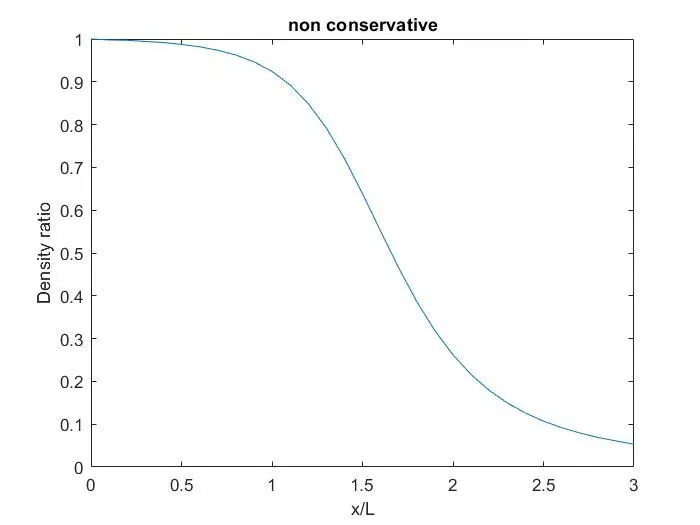
- It can be observed that the density ratio decreases on each successive grid points
Pressure ratio W.r.t X
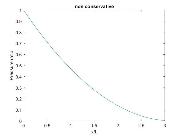
- Pressure ratio seems to be decreasing on each grid point and at the exit it approaches 0
Temperature ratio vs X
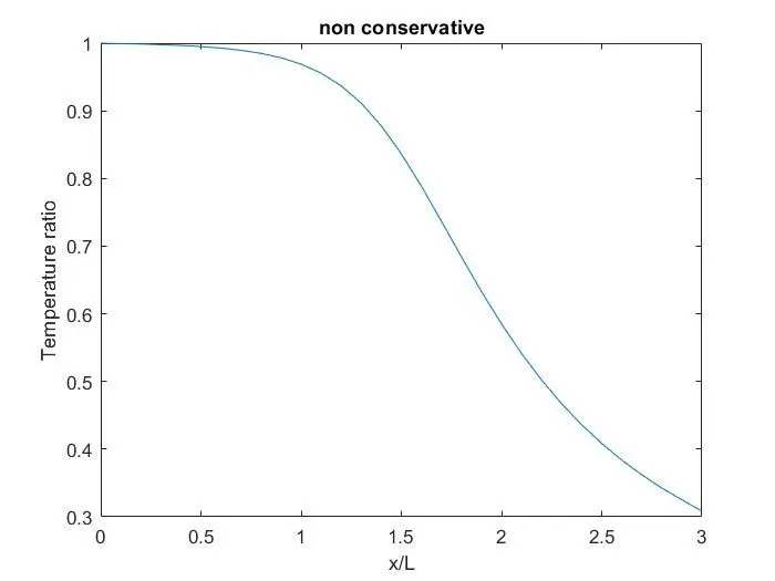
- Temperature ratio decreases upto a value around 0.3 at exit
Velocity ratio vs X
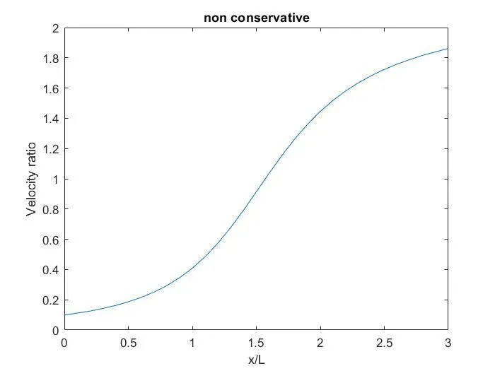
- Velocity ratio is getting increased when passed through the nozzle, indicating velocity at each point is increasing
Mach number vs X
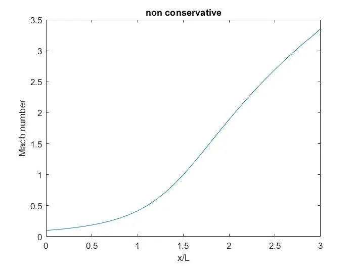
- Mach number increases when moved through the nozzle
Mass flow rate vs X
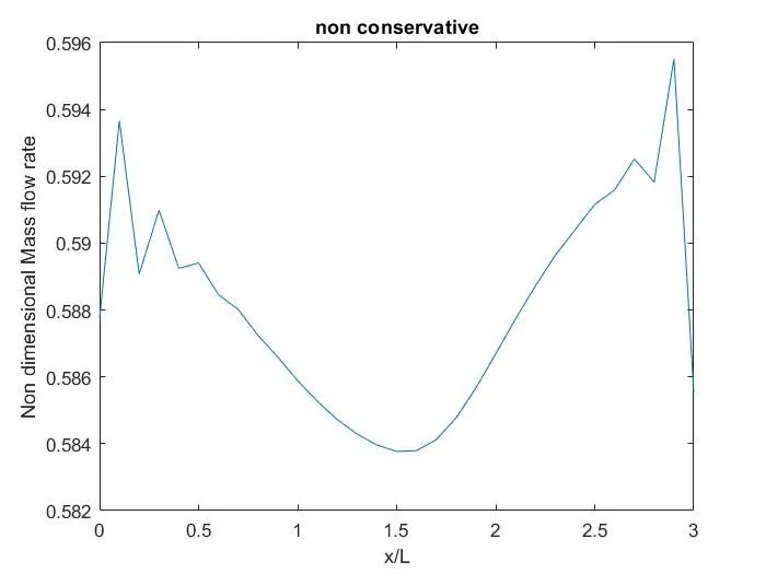
- There is a sudden increase in mass flow rate at entry and at exit there is a sudden drop . Also at throat the mass floow rate is comparitively low.
Throat values
Density ratio vs time steps
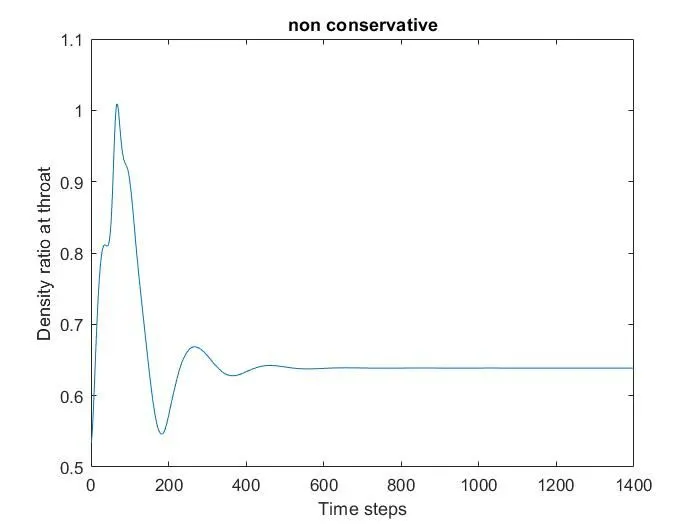
- At around 500th iterations the value becomes stable
Velocity ratio vs time steps
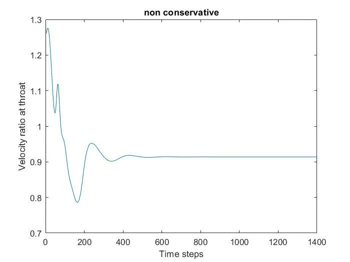
- At around 500th iterations the value becomes stable
Pressure ratio vs time steps
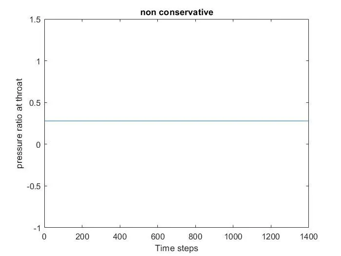
- The value is constant across all iterations
Temperature ratio vs time steps
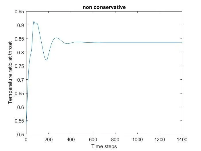
- At around 500th iterations the value becomes stable
Mach number vs time steps
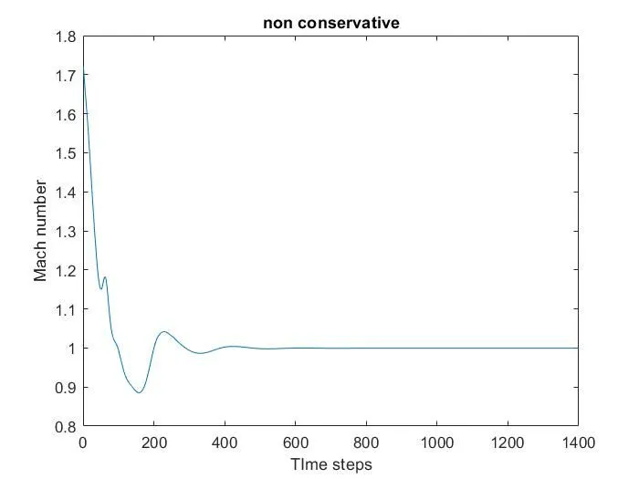
- At around 500th iterations the value becomes stable
Mass flow rate
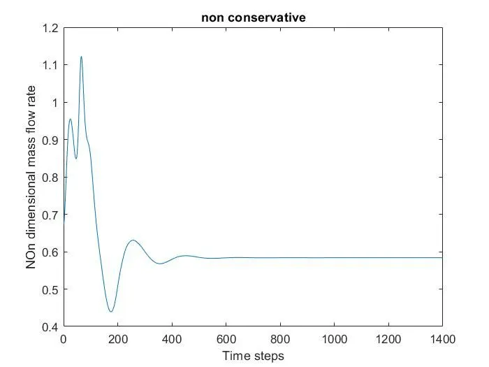
- At around 500th iterations the value becomes stable
Conservative form
Continuity equation
`(del(rho*A'))/(delt') + (del(rhoAV'))/(delx') = 0`
Momentum equation
`(del(rhoAV'))/(delt') + (del(rhoAV^2))/(delx) = -A(delP)/(delx)`
Energy equation
`(del(rhoA))/(delt') + (del(rhoeV'A'))/(delx') = -P(del(AV))/(delx)`
The above form of equations are converted to simpler form for an efficient calculation. It is done by replacing some terms as follows
Solution vectors
U1 = `rho'A'`
U2 = `rho'A'V'`
U3 = `rho'((e')/(gamma-1) + (gamma/2)V^2)A'`
Flux vectors
F1 = `rho'A'V'`
F2 = `rho'A'V'^2 + (1/gamma)P'A'`
F3 = `rho(e/(gamma-1)+gamma/2V^2)+rhoAV`
Source vectors
J2 = `1/gammarho(delA)/(delx)`
So the transformed equations will be
Continuety equation
`(delU1)/(delt) = -(delF1)/(delx`
Momentum equation
`(delU2)/(delt) = -(delF2)/(delx) + J2`
Energy equation
`(delU3)/(delt) = -(delF3)/(delx`
we follow the same procedure like we did in non-conservative method, so for computation we will have these three parts
- Predictor step
- Corrector step
- Avarage step
Predictor step
Here we will do Forward differencing scheme
Continuity equation
`(delU1)/(delx_p)(j) = -(F1(j+1)-F1(j))/dx;`
Momentum equation
`(delU2)/(delx_p)(j) = -(F2(j+1)-F2(j))/dx + J2(j);`
`J2(j) = (gamma)^-1 * rho(j)*T(j)*(a(j+1)-a(j))/dx;`
Energy equation
`(delU3)/(delx_p)(j) = -(F3(j+1)-F3(j))/dx;`
After this we have to update each solution vectors in the same for like we did in non-conservstive form
`U1(j) = U1(j)+(delU1)/(dx_p)(j)*dt`
`U2(j) = U2(j)+(delU2)/(dx_p)(j)*dt`
`U3(j) = U3(j)+(delU3)/(dx_p)(j)*dt`
- Then we will define premitive values
`rho = U_1/A;`
`V = U_2/U_1;`
`T= (gamma-1)*((U_3/U_1)-0.5*r*v^2)`
`p = rho*T`
- Then the flux vectors are updated
F1 = U2;
`F2 = ((U2^2)/(U1))+((gamma-1)/gamma)*(U3-((gamma/2)*((U2^2)/(U1))));`
`F_3 = (gamma*U_2*(U_3)/(U_1))-(gamma*(gamma-1)/2)*(U_2^3/U_1^2);`
Corrector step
Here we will use backward differencing scheme
So the equations are discretized as follows
Continuity equation,
`(delU1)/(delx_c)(j) = -(F1(j)-F1(j-1))/dx;`
Momentum equation,
`(delU2)/(delx_c)(j) = -(F2(j+1)-F2(j))/dx + J2(j)`
`J2(j) = (gamma)^-1 * rho(j)*T(j)*(a(j)-a(j-1))/dx;`
Energy equation,
`(delU3)/(delx_c)(j) = -(F3(j+1)-F3(j))/dx;`
Avarage step
`(delU_1)/(delx_(avg)) = 0.5*((delU_1)/(delx_p) + (delU_1)/(delx_c));`
`(delU_2)/(delx_(avg)) = 0.5*((delU_2)/(delx_p) + (delU_2)/(delx_c));`
`(delU_3)/(delx_(avg)) = 0.5*((delU_3)/(delx_p) + (delU_3)/(delx_c));`
So using the avarage step we update the values again for U1,U2,U3 (like before) and this will be our final update, so using these new values we update the values for rho,T,v, as well.
Code
%conservative
close all
clear all
clc

n = 31;
x = linspace (0,3,n);
dx = x(2)-x(1);
r =1.4; %gamma
C = 0.5; %CFL number
%Shape of nozzle
a = 1+2.2.*(x-1.5).^2;

for i = 1:length(x)

%initial conditions
if x(i)>=0 && x(i)< 0.5
    rho(i) = 1;
    T(i) = 1;
elseif x(i)>=0.5 && x(i)<1.5
    rho(i) = 1-0.366.*(x(i)-0.5);
    T(i) = 1-0.167.*(x(i)-0.5);
elseif x(i) >= 1.5 && x(i)< 3.5
    rho(i) = 0.634-0.3879.*(x(i)-1.5);
    T(i) = 0.833-0.3507.*(x(i)-1.5);
end
end
%primitive variables
v = 0.59./(rho.*a);
p = rho.*T;


%solution vectors
U1 = rho.*a;
U2 = rho.*a.*v ;
U3 = rho .*(T/(r-1) + 0.5*r*v.^2).*a;
%time loop
nt = 1400;
iteration = 1;
%predictor step
tic
for k= 1:nt
    %creating a copy of solution vector
    U1_old = U1;
    U2_old = U2;
    U3_old = U3;

    %time step
    dt = min((C*dx)./(realsqrt(T)+v));
    %flux vectors
    F1 = U2;
    F2 = ((U2.^2)./U1)+((r-1)/r).*(U3-((r/2)*(U2.^2./U1)));
    F3 = (r.*U2.*U3./U1)-(r*(r-1)/2)*(U2.^3./U1.^2);

    for j = 2:n-1
        J2(j) = (r)^-1 .* rho(j).*T(j).*(a(j+1)-a(j))/dx;
        dU1dx_p(j) = -(F1(j+1)-F1(j))/dx;
        dU2dx_p(j) = -(F2(j+1)-F2(j))/dx + J2(j);
        dU3dx_p(j) = -(F3(j+1)-F3(j))/dx;

        %updating values for solution vectors
        U1(j) = U1(j)+(dU1dx_p(j)).*dt;
        U2(j) = U2(j) + (dU2dx_p(j)).*dt;
        U3(j) = U3(j) + (dU3dx_p(j)).*dt;
    end

    %updting the primitive values
    rho = U1./a;
    v = U2./U1;
    T= (r-1).*((U3./U1)-0.5.*r.*v.^2);
    p = rho.*T;

     %Updating the flux vectors
    F1 = U2;
    F2 = (U2.^2./U1)+((r-1)/r)*(U3-((r/2)*(U2.^2./U1)));
    F3 = (r.*U2.*U3./U1)-(r*(r-1)/2)*(U2.^3./U1.^2);

    %corrector step
    for j = 2:n-1
%        J2(j) = (r)^-1 .* rho(j).*T(j).*(a(j+1)-a(j))/dx;
        J2(j) = (r)^-1 .* rho(j).*T(j).*(a(j)-a(j-1))/dx;
        dU1dx_c(j) = -(F1(j)-F1(j-1))/dx;
        dU2dx_c(j) = -(F2(j)-F2(j-1))/dx + J2(j);
        dU3dx_c(j) = -(F3(j)-F3(j-1))/dx;
    end

    %finding the avarage
     dU1dx_avg = 0.5.*(dU1dx_p + dU1dx_c);
    dU2dx_avg = 0.5.*(dU2dx_p + dU2dx_c);
    dU3dx_avg = 0.5.*(dU3dx_p + dU3dx_c);

     for m =2:n-1
        %updating values for solution vectors
        U1(m) = U1_old(m)+ (dU1dx_avg(m)).*dt;
        U2(m) = U2_old(m) + (dU2dx_avg(m)).*dt;
        U3(m) = U3_old(m) + (dU3dx_avg(m)).*dt;
     end
    iteration = iteration + 1;
    %boundary conditions
    %Subsonic Inflow(point 1)
    U1(1) = (rho(1).*a(1));
    U2(1) = 2.*U2(2)-U2(3);
    U3(1) = U1(1).*((T(1)/(r-1))+0.5*r.*v(1).^2);

    %Supersonic outflow(pointN)
    U1(n) = 2.*(U1(n-1))-U1(n-2);
    U2(n) = 2.*(U2(n-1))-U2(n-2);
    U3(n) = 2.*(U3(n-1))-U3(n-2);


    %updting the primitive values at exit
    rho = U1./a;
    v = U2./U1;
    T= (r-1).*((U3./U1)-0.5.*r.*v.^2);
    p = rho.*T;
    mfr=rho.*v.*a;
    Mach_number = v./(T.^0.5)

    %for mass flow rate at each time step
figure(1)
if k==50
    figure(1)
    plot(x,mfr,'color','r')

    hold on
elseif k==100
    figure(1)
    plot(x,mfr,'color','g')
    hold on
elseif k==200
    figure(1)
    plot(x,mfr,'color','b')

    hold on
elseif k==500
    figure(1)
    plot(x,mfr,'color','c')

    hold on
else if k==700
    figure(1)
    plot(x,mfr,'color','m')

elseif k==1400
    figure(1)
    plot(x,mfr,'color','k')
    xlabel('x/L')
    ylabel('Mass flow rate')
    legend ('50th Time step', '100th time step','200th time step','500th time step','700th time step','1400th time step')
    end
end

    % Throat variables.
    T_throat(k)=T(16);
    v_throat(k)=v(16);
    rho_throat(k)=rho(16);
    p_throat(k)=p(16);
    M_throat(k) = Mach_number(16);
    mfr_throat(k) = mfr(16);

end

Elapsed_time = toc;

figure(2)
plot(p_throat)
xlabel('Time steps')
ylabel('pressure ratio at throat')
title('conservative')

figure(3)
plot(T_throat)
xlabel('Time steps')
ylabel('Temperature ratio at throat')
title('conservative')

figure(4)
plot(rho_throat)
xlabel('Time steps')
ylabel('Density ratio at throat')
title('conservative')

figure(5)
plot(v_throat)
xlabel('Time steps')
ylabel('Velocity ratio at throat')
title('conservative')

figure(6)
plot(x,T)
xlabel('x/L')
ylabel('Temperature ratio')
title('conservative')

figure(7)
plot(x,p)
xlabel('x/L')
ylabel('Pressure ratio')
title('conservative')

figure(8)
plot(x,v)
xlabel('x/L')
ylabel('Velocity ratio')
title('conservative')

figure(9)
plot(x,rho)
xlabel('x/L')
ylabel('Density ratio')
title('conservative')

figure(10)
plot(x,mfr)
xlabel('x/L')
ylabel('Non dimensional Mass flow rate')
title('conservative')

figure(11)
plot(x,Mach_number)
xlabel('x/L')
ylabel('Mach number')
title('conservative')

figure(12)
plot(mfr_throat)
xlabel('Time steps')
ylabel('Non dimensional mass flow rate')
title('conservative')

figure(13)
plot(M_throat)
xlabel('TIme steps')
ylabel('Mach number')
title('conservative')
Elapsed_time = 11.0347
Obtained plots
Velocity ratio vs non dimensional grid (x')
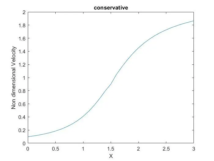
-
- Velocity ratio is getting increased when passed through the nozzle, indicating velocity at each point is increasing
Temperature ratio vs non dimensional grid (x')
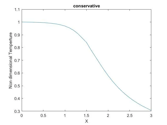
- Temperature ratio decreases upto a value around 0.3 at exit
Pressure ratio vs non dimensional grid (x')
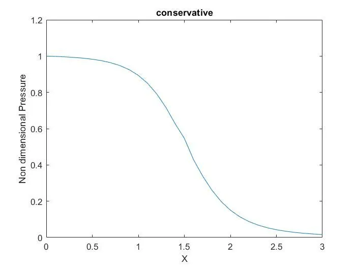
Pressure ratio seems to be decreasing on each grid point and at the exit it approaches 0
Density ratio vs non dimensional grid (x')
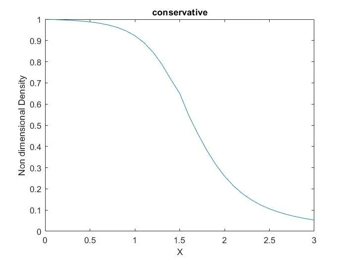
- It can be observed that the density ratio decreases on each successive grid points
Mass flow rate vs non dimensional grid (x')
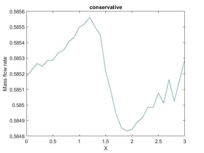
- Mass flow rate seems to be in an increasing manner up until where x is between 1 and 1.5 then it decreases to a lower value and gets increased at exit
Mach number vs non dimensional grid (x')
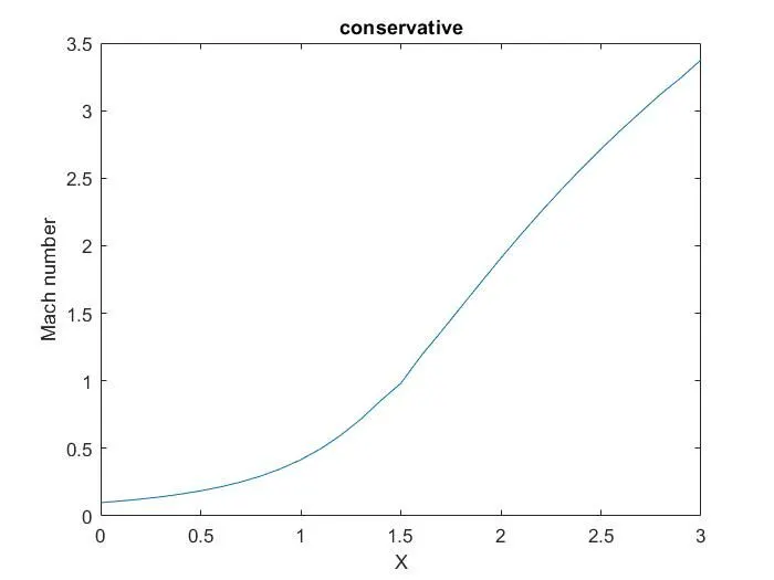
- Mach number is increasing across the nozzle and it is higher at exit
Throat values
Velocity ratio vs Time steps (nt)
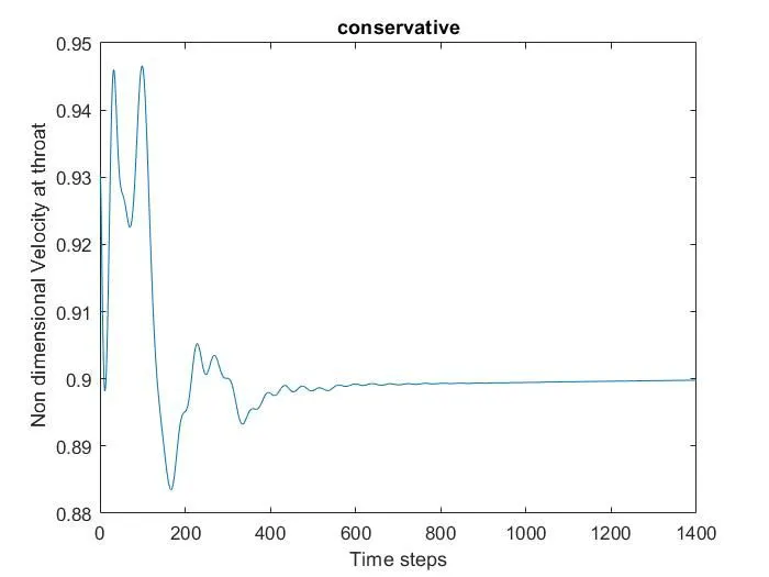
- A stable solution is obtained around 600th iterations
Pressure ratio vs Time steps (nt)
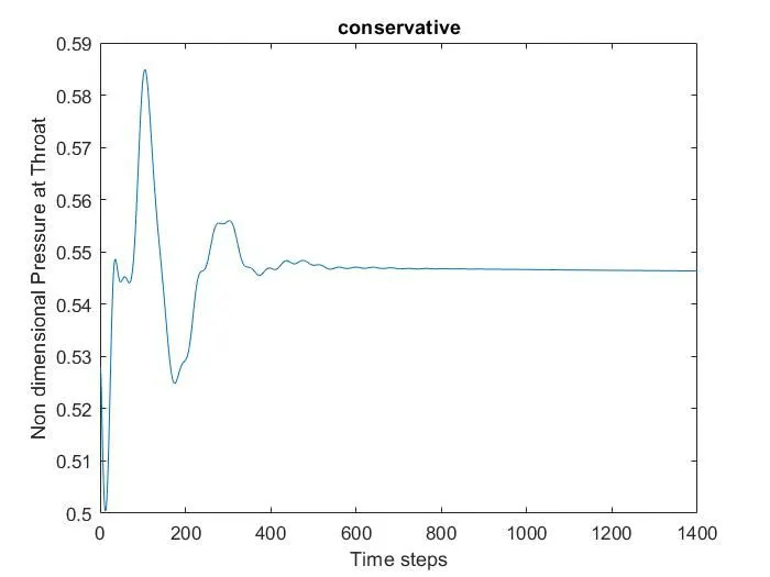
- A stable solution is obtained around 600th iterations
Temperature ratio vs Time steps (nt)
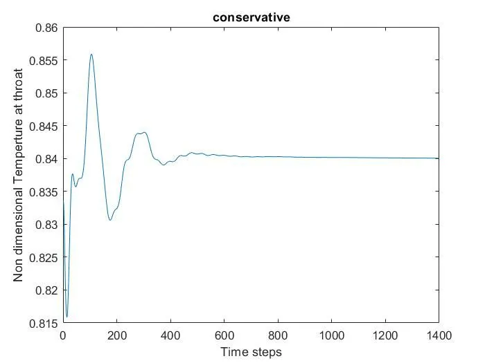
- A stable solution is obtained around 700th iterations
Density ratio vs Time steps (nt)
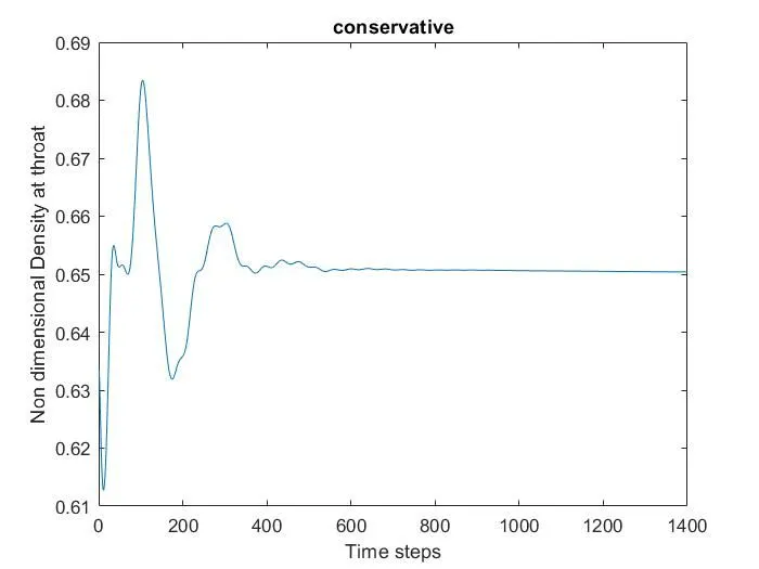
- A stable solution is obtained around 700th iterations
Mach number vs Time steps (nt)
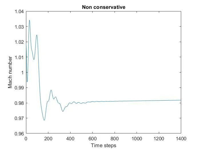
- A stable solution is obtained around 700th iterations
Mass flow rate vs Time steps (nt)
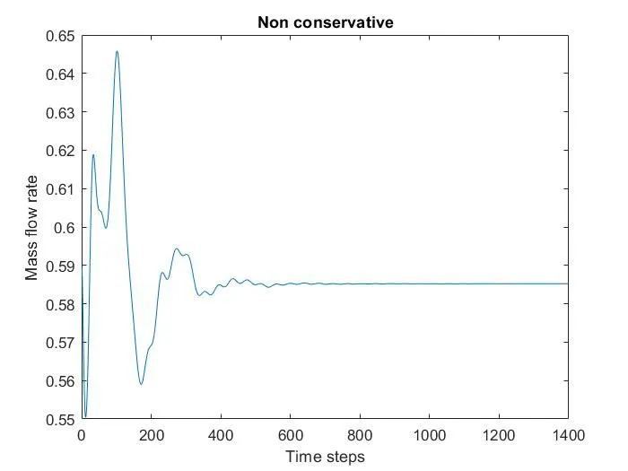
- A stable solution is obtained around 700th iterations
Grid independence study
| Conservational Form | Non-conservational form | ||||||||||||||||||||||||||||||
|
|
- Let us take a look at the table listed above, I have listed the values of non dimensional pressure , Temperature, Velocity,Density from both conservative and non conservative method at inlet and exit with different number of grid points to study the grid independence study
- There is no much difference from the values when the grid numbers are changing, or there is only a small difference in values so we can say that when grid numbers increase solution accuracy also increases
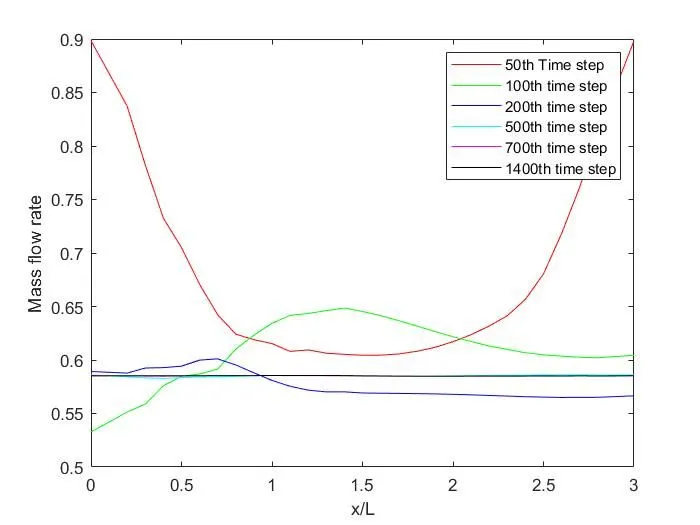
Comparison of non dimensional mass flow rate at different time steps for conservative form and non-conservative form
Conservative form
Non-conservative form
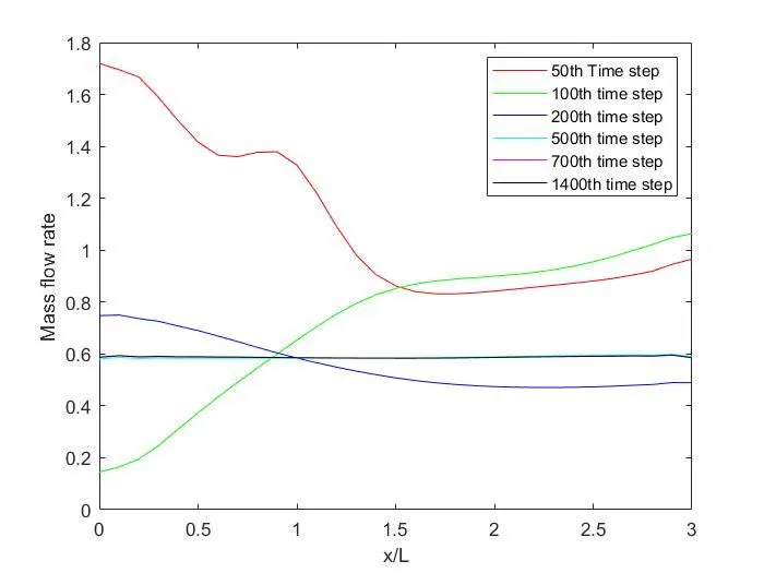
- It can be seen that at initial stages of itrations we have different curves on conservative and non conservative form
- But after 500th iterations both the curves appears to be similiar
- That is we will have a stable solution after 500th iterations
Comparison of Normalized mass flow rate distributions of both forms
Code
%mass flow rate values obtained from non-conservative solution
mfr = [0.587751927825053,0.593661417754617,0.589074692600847,0.590986115492168,0.589248097068662,0.589408285785002,0.588461074417405,0.588016825837875,0.587240313719640,0.586592511541659,0.585883701555310,0.585265340319724,0.584720320434025,0.584288706983882,0.583961297675112,0.583768589264520,0.583793288791218,0.584123134615336,0.584773405890310,0.585667748625384,0.586688164447450,0.587732779668089,0.588716695016250,0.589630599522300,0.590395293944765,0.591157131254359,0.591589221986176,0.592516257548227,0.591827391902550,0.595513246311297,0.585534812613340];
%mass flow rate values obtained from conservative solution
mfr_c = [0.585182570170289,0.585223985421496,0.585265400672702,0.585248250843886,0.585285099361468,0.585287560301832,0.585333137419525,0.585349835329159,0.585404076716080,0.585433380792077,0.585498421326970,0.585519406852654,0.585561311741159,0.585498823883350,0.585448681365884,0.585216997541020,0.585084599642513,0.584938999301107,0.584852438245619,0.584832768234162,0.584843467130633,0.584890630879243,0.584918539070959,0.584985832906570,0.584983744041948,0.585077065656957,0.585011386275988,0.585161398757709,0.585024375282778,0.585156569538446,0.585288763794114];
%grid
x= linspace(0,3,31)

%plotting
plot(x,mfr)
hold on
plot(x,mfr_c)
xlabel('x/L')
ylabel('Non dimensional mass flow rate')
legend('non conservative','conservative')
Obtained plot
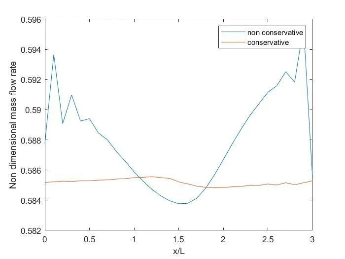
- It is clear that the conservative form takes less deviation, that is it shows more stable solution than the non-conservative form
Conclusions
- From the above informations it is clear that the difference between conservative solution and non-conservative solution are very small
- Although we have seen that the time required to compute the problem had a defference in both forms. Out of which the conservative form had the superiority as it took less time to compute. Conservative form only took 11 seconds whereas the non-conservative form took 26 seconds
- There was no much of a difference seen when the primitive variables (graphs) were compared from both forms
- Throat values with respct to time steps from both forms where compared and it was noted that the non-conservative part showed constant values after 500th iteration while th conservative part took around 600 to 700th iterations which was the only noted difference