Week 3.5 - Deriving 4th order approximation of a 2nd order derivative using Taylor Table method

We use taylor table to find the higher order approximations. This table is designed in a way to take out the terms and use it effectively to find out the coefficients. Suppose we want to find fourth order approximation of a second order derivative. We can find it using the information from the neighbouring points. We can solve this by using these three techniques .

1. Central differencing

2. Skewed-right sided differencing

3. skewed-left sided differencing

1. Central differencing Method

Since this is a symmetric scheme,

P = N-Q+1

P = Order of accuracy we want = 4

N= Number of nodes

Q = Order of derivative = 2

Therefore the number of nodes to be takes are 5. ie, two nodes from right side and two from left side.

	f(i)	`Deltax*f'(i)`	`Deltax^2*f''(i)`	`Deltax^3*f'''(i)`	`Deltax^4*f''''(i)`	`Deltax^5*f'''''(i)`	`Deltax^6*f''''''(i)`
a*f(i-2)	a	-2a	2a	-8a/6	16a/24	-32a/120	64a/720
b*f(i-1)	b	-b	b/2	-b/6	b/24	-b/120	b/720
c*f(i)	c	0	0	0	0	0	0
d*f(i+1)	d	d	d/2	d/6	d/24	d/120	d/720
e*f(i+2)	e	2e	2e	8e/6	16e/24	32e/120	64e/720
`Sigma`	0	0	1	0	0	?	?

1) a+b+c+d+e = 0

2) -2a-b+d+2e = 0

3) 2a+b/2+d/2+2e = 1

4) -8a/6 - b/6 + d/6+8e = 0

5) 16a/24 + b/24 + d/24 + 16e/24 = 0

Now we have five unknowns and five equations so we use matrix to determine the value of each unknown

When written in matrix form

`[[1, 1, 1, 1, 1],[-2, -1, 0, 1, 2],[4/2, 1/2, 0, 1/2, 4/2],[-8/6, -1/6, 0, 1/6, 8/6],[16/24, 1/24, 0, 1/24, 16/24],[-32/120, -1/120, 0, 1/120, 32/120]][[a],[b],[c],[d],[e]]=[[0],[0],[1],[0],[0]]`

Solving above linear equations using Matlab

%matrix A
A = [1,1,1,1,1;-2,-1,0,1,2;2,1/2,0,1/2,2;-8/6,-1/6,0,1/6,8/6;16/24,1/24,0,1/24,16/24];
%matrix B
B= [0;0;1;0;0];

C = A\B

Solution obtained

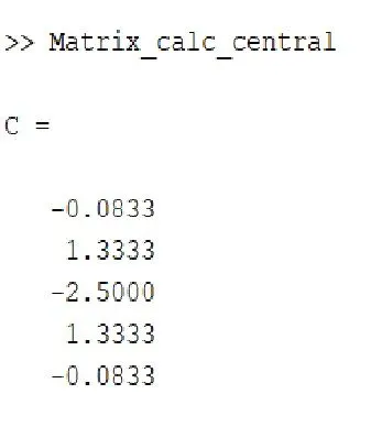
ie, a = -0.0833

b = 1.3333

c = -2.5

d = 1.3333

e = -0.0833

So the equation can be written as

`(del^2y)/(delx^2)=(af(i-2)+bf(i-1)+cf(i)+df(i+1)+ef(i+2))/(Deltax^2)`

2) Skewed right-sided differencing

Since this is an asymmetric scheme,

P = N-Q

P = Order of accuracy we want = 4

N= Number of nodes

Q = Order of derivative = 2

Therefore the number of nodes to be takes are 6. ie, 5 nodes from right side .

	f(i)	`Deltax*f'(i)`	`Deltax^2*f''(i)`	`Deltax^3*f'''(i)`	`Deltax^4*f''''(i)`	`Deltax^5*f'''''(i)`	`Deltax^6*f''''''(i)`
a*f(i)	a	0	0	0	0	0	0
b*f(i+1)	b	b	b/2	b/6	b/24	b/120	b/720
c*f(i+2)	c	2c	2c	8c/6	16c/24	32c/120	64c/720
d*f(i+3)	d	3d	9d/2	27d/6	81d/24	243d/120	729d/720
e*f(i+4)	e	4e	8e	64e/6	256e/24	1024e/120	4096e/720
g*f(i+5)	g	5g	25g/2	125g/6	625g/24	3125g/120	15625g/720
`Sigma`	0	0	1	0	0	0	?

1. a+b+c+d+e+g = 0

2. b+2c+3d+4e+5g = 0

3. b/2+2c+9d/2+8e+ 25g/2 = 1

4. b/6+8c/6+27d/6+64e/6+125g/6 = 0

5. b/24+16c/24+81d/24+256e/24+625e/24 = 0

6. b/120+32c/120+243d/120+1024e/120+3125g/120 = 0

When written in matrix form

`[[1, 1, 1, 1, 1, 1],[0, 1, 2, 3, 4, 5],[0, 1/2, 2, (9)/2, 8, (25)/2],[0, 1/6, (8)/6, (27)/6, (64)/6, (125)/6],[0, 1/24, (16)/24, (81)/24, (256)/24, (625)/24],[0, 1/120, (32)/120, (243)/120, (1024)/120, (3125)/120]][[a],[b],[c],[d],[e],[g]]=[[0],[0],[1],[0],[0],[0]]`

So the above matrices is in linear form which can solved through matlab as shown below

%matrix A
A = [1,1,1,1,1,1;0,1,2,3,4,5;0,1/2,2,9/2,8,25/2;0,1/6,8/6,27/6,64/6,125/6;0,1/24,16/24,81/24,256/24,625/24;0,1/120,32/120,243/120,1024/120,3125/120]
%matrix B
B = [0;0;1;0;0;0]
%solution
X = A\B

Solution obtained

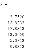
ie, a = 3.75

b = -12.833

c = 17.8333

d = -13

e = 5.0833

g = -0.833

So the equation can be written as

`(del^2y)/(delx^2)=(af(i)+bf(i+1)+cf(i+2)+df(i+3)+ef(i+4)+gf(i+5))/(Deltax^2)`

3) Skewed left-sided differencing

Since this is an asymmetric scheme,

P = N-Q

P = Order of accuracy we want = 4

N= Number of nodes

Q = Order of derivative = 2

Therefore the number of nodes to be takes are 6. ie, 5 nodes from left side .

	f(i)	`Deltax*f'(i)`	`Deltax^2*f''(i)`	`Deltax^3*f'''(i)`	`Deltax^4*f''''(i)`	`Deltax^5*f'''''(i)`	`Deltax^6*f''''''(i)`
a*f(i)	a	0	0	0	0	0	0
b*f(i-1)	b	-b	b/2	-b/6	b/24	-b/120	b/720
c*f(i-2)	c	-2c	2c	-8c/6	16c/24	-32c/120	64c/720
d*f(i-3)	d	-3d	9d/2	-27d/6	81d/24	-243d/120	729d/720
e*f(i-4)	e	-4e	8e	-64e/6	256e/24	-1024e/120	4096e/720
g*f(i-5)	g	-5g	25g/2	-125g/6	625g/24	-3125g/120	15625g/720
`Sigma`	0	0	1	0	0	0	?

1. a+b+c+d+e+g = 0

2. -b-2c-3d-4e-5g = 0

3. b/2+2c+9d/2+8e+ 25g/2 = 1

4. -b/6-8c/6-27d/6-64e/6-125g/6 = 0

5. b/24+16c/24+81d/24+256e/24+625e/24 = 0

6. -b/120-32c/120-243d/120-1024e/120-3125g/120 = 0

When written in matrix form,

`[[1, 1, 1, 1, 1, 1],[0, -1, -2, -3, -4, -5],[0, 1/2, 2, (9)/2, 8, (25)/2],[0, -1/6, -(8)/6, -(27)/6, -(64)/6, -(125)/6],[0, 1/24, (16)/24, (81)/24, (256)/24, (625)/24],[0, -1/120, -(32)/120, -(243)/120, -(1024)/120, -(3125)/120]][[a],[b],[c],[d],[e],[g]]=[[0],[0],[1],[0],[0],[0]]`

This is solved using matlab

%matrix A 
A = [1, 1, 1, 1, 1, 1;0, -1, -2, -3, -4, -5;0, 1/2, (4)/2, (9)/2, (16)/2, (25)/2;0, -1/6, -(8)/6, -(27)/6, -(64)/6, -(125)/6;0, 1/24, (16)/24, (81)/24, (256)/24, (625)/24;0, -1/120, -(32)/120, -(243)/120, -(1024)/120, -(3125)/120]
%matrix B
B = [0;0;1;0;0;0]
%solution
X = A\B

Obtained solution

ie, a = 3.75

b = -12.833

c = 17.8333

d = -13

e = 5.0833

g = -0.833

So the equation can be written as

`(del^2y)/(delx^2)=(af(i)+bf(i-1)+cf(i-2)+df(i-3)+ef(i-4)+gf(i-5))/(Deltax^2)`

Function for central differencing

function [out]=central_difference(x,dx)
% a = -0.0833;
% b = 1.333   ;
% c = -2.5;
% d = 1.3333;
% e = -0.0833;
a=-5/60;
b=4/3;
c=-2.5;
d=4/3;
e=-5/60;
analytical_derivative =-2*exp(x)*sin(x);
central_numerical_derivative =((a*((exp(x-(2*dx))*cos(x-(2*dx)))))+(b*((exp(x-dx)*cos(x-dx))))+(c*(exp(x)*cos(x)))+(d*((exp(x+(dx))*cos(x+(dx)))))+(e*((exp(x+(2*dx)))*cos(x+(2*dx)))))/((dx)^2);
out=abs(analytical_derivative-central_numerical_derivative);
end

Function for skewed right sided

function [out] = skewed_right_sided_differencing(x,dx)
%a = 3.75
%b = -12.833
%c = 17.8333
%d = -13
%e = 5.0833
%g = -0.833
a=15/4;
b=-77/6;
c=107/6;
d=-13;
e=61/12;
g =-5/6
analytical_derivative =-2*exp(x)*sin(x);
skewed_right_numerical_derivative =((a*((exp(x)*cos(x))))+(b*((exp(x+dx)*cos(x+dx))))+(c*(exp(x+2*dx)*cos(x+2*dx)))+(d*((exp(x+(3*dx))*cos(x+(3*dx)))))+(e*((exp(x+(4*dx)))*cos(x+(4*dx))))+(g*((exp(x+(5*dx)))*cos(x+(5*dx)))))/((dx)^2);
out=abs(analytical_derivative-skewed_right_numerical_derivative)
end

Function for left sided differencing

function [out] = left_sided_differencing(x,dx)
%a = 3.75
%b = -12.833
%c = 17.8333
%d = -13
%e = 5.0833
%g = -0.833
a=15/4;
b=-77/6;
c=107/6;
d=-13;
e=61/12;
g=-5/6
analytical_derivative =-2*exp(x)*sin(x);
skewed_left_numerical_derivative =((a*((exp(x)*cos(x))))+(b*((exp(x-dx)*cos(x-dx))))+(c*(exp(x-2*dx)*cos(x-2*dx)))+(d*((exp(x-(3*dx))*cos(x-(3*dx)))))+(e*((exp(x-(4*dx)))*cos(x-(4*dx))))+(g*((exp(x-(5*dx)))*cos(x-(5*dx)))))/((dx)^2);
out=abs(analytical_derivative-skewed_left_numerical_derivative)
end

Main code

close all
clear all
clc

%Given function f(x) = exp(x).cos(x)
%analytical derivative = -2*exp(x)*sin(x
%Numerical derivative through central differencing
%(a*f(i-2)+b*f(i-1)+c(i)+d*f(i+1)+e*f(i+2))/(dx)^2;
x = pi/3;
dx= linspace(pi/40,pi/4000,20);
for i=1:length(dx)
    error_central(i)=central_difference(x,dx(i));   %calling the function
    error_right_sided(i)=skewed_right_sided_differencing(x,dx(i));  %calling the function
    error_left_sided(i)=left_sided_differencing(x,dx(i));  %calling the function



end
loglog(dx,error_central,'r')
hold on
loglog(dx,error_right_sided,'b')
hold on
loglog(dx,error_left_sided,'g')
xlabel('Range of dx')
ylabel('error')
legend('Error of central differencing','Error of skewed right sided differencing','Error of skewed left sided')

Plotting

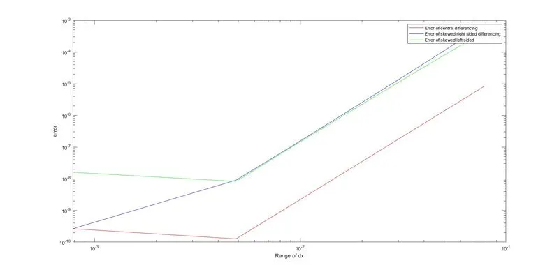
We can see that after some particular points in dx the error goes in an increasing manner , this is becouse of the round of error occur due to computational limits

Why Skewed scheme is more useful than a central differencing scheme

Although the error shown in Cental differencing scheme is less skewed scheme is useful in most of the cases .Its just becouse we need informations from both right side and left side for a central differencing scheme where as in skewed schem we need only information from one side, either left or right.