Week 9 - FVM Literature Review
Finite Volume Method
- The finite volume method (FVM) is a method for representing and evaluating partial differential equations in the form of algebraic equations.
- In the finite volume method, volume integrals in a partial differential equation that contain a divergance term are converted to surface integrals, using the divergance theorem.
- These terms are then evaluated as fluxes at the surfaces of each finite volume. Because the flux entering a given volume is identical to that leaving the adjacent volume, these methods are conservative.
- Another advantage of the finite volume method is that it is easily formulated to allow for unstructured meshes.
- The method is used in many CFD packages.
- "Finite volume" refers to the small volume surrounding each node point on a mesh.
Major differences between FDM & FVM
- FDM is a differential scheme, that is approximation of a taylor series expansion.You try to write the first order, second order differential in terms of difference between two point values. This may bring in some approximation error.
- Finite Volume method is an integral scheme. Since you are integrating across the area, chance of error is minimized.
-
Differential schemes are faster and error can be minimized if you have regular grids (squares and rectangles).
-
Integral schemes are slightly slower but score over FDM when the mesh is irregular.
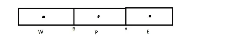
- Since east term is used to find the east phase and `alpha`is a function of temperature we need to find the values of temperature in east phase. Inorder to do that we need to have some kind of interpolation schemes
Type of interpolation schemes
1. Upwind interpolation shceme
Is same as the forward differencing scheme , it uses node values at upwind to interpolate the results
2.Linear interpolation scheme
Linear interpolation is a method of curve fitting using linear polynomials to construct new data points within range of a discrete set of known data points.
3.Quadratic interpolation scheme
Is the process of using second order polynomial to make interpolation for a function and it requires the existance of three points.
4.Hybrid interpolation scheme
This scheme is the combination of Upwind interpolation and linear interpolation scheme.
Flux limiters
Flux limiters are used in high resolution schemes – numerical schemes used to solve problems in science and engineering, particularly fluid dynamics, described by partial differential equations (PDE's). They are used in high resolution schemes, such as the MUSCL scheme, to avoid the spurious oscillations (wiggles) that would otherwise occur with high order spatial discretization schemes due to shocks, discontinuities or sharp changes in the solution domain. Use of flux limiters, together with an appropriate high resolution scheme, make the solutions more accurate.
Working
The main idea behind the construction of flux limiter schemes is to limit the spatial derivatives to realistic values – for scientific and engineering problems this usually means physically realisable and meaningful values. They are used in high resolution schemes for solving problems described by PDEs and only come into operation when sharp wave fronts are present. For smoothly changing waves, the flux limiters do not operate and the spatial derivatives can be represented by higher order approximations without introducing spurious oscillations.

where and
and  represent edge fluxes for the ith cell. If these edge fluxes can be represented by low and high resolution schemes, then a flux limiter can switch between these schemes depending upon the gradients close to the particular cell, as follows,
 ,
, ,
,
where
 low resolution flux,
 high resolution flux,
 flux limiter function,
and `phi(r)` represents the ratio of successive gradients on the solution mesh, i.e.,
 .
.
The limiter function is constrained to be greater than or equal to zero, i.e.,  . Therefore, when the limiter is equal to zero (sharp gradient, opposite slopes or zero gradient), the flux is represented by a low resolution scheme. Similarly, when the limiter is equal to 1 (smooth solution), it is represented by a high resolution scheme. The various limiters have differing switching characteristics and are selected according to the particular problem and solution scheme. No particular limiter has been found to work well for all problems, and a particular choice is usually made on a trial and error basis.