Week - 9 Material Modeling from Raw Data
Aim:
To create a material card using the data which is extracted from the given true stress-strain curve in the model for graphite iron casting
and assign it to the given dog bone specimen.
1.Extract the data from the given curve.
2.Clean the data and verify it with the original given data and the given elastic modulus is20.9E+06 psi.
3.Convert the data to (kg-mm-ms) unit system.
4.Process the data and create the material as demonstrated.
5.Use the material model with a dogbone specimen and validate the same.
Procedure:
1.The given image file of stress-strain curve of the given graphite iron casting is imported into the data digitizer software to extract the data and
export it as excel file.
From the fig we taken the curve 2 to extract the data.
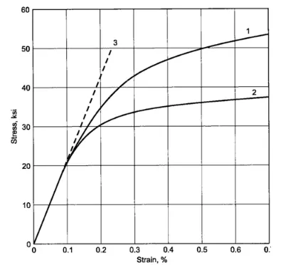
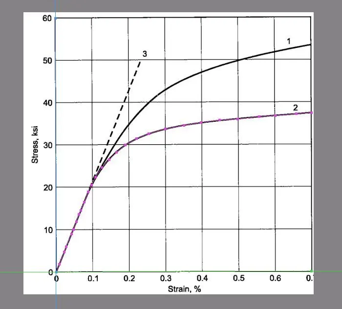
Fig:Image and points for data extractions.
Mat curve 2
| Strain % | True strain | Stress ksi |
| 0.00851 | 0.0000851 | 1.87E+00 |
| 0.0219 | 0.000219 | 4.67 |
| 0.028 | 0.00028 | 6.02 |
| 0.0425 | 0.000425 | 9.03 |
| 0.0474 | 0.000474 | 10.1 |
| 0.0559 | 0.000559 | 11.8 |
| 0.0632 | 0.000632 | 13.6 |
| 0.0681 | 0.000681 | 14.5 |
| 0.0778 | 0.000778 | 16.5 |
| 0.0887 | 0.000887 | 18.9 |
| 0.0972 | 0.000972 | 2.06E+01 |
| 0.108 | 0.00108 | 22.3 |
| 0.126 | 0.00126 | 24.7 |
| 0.146 | 0.00146 | 26.6 |
| 0.166 | 0.00166 | 28.2 |
| 0.19 | 0.0019 | 30 |
| 0.222 | 0.00222 | 31.4 |
| 0.256 | 0.00256 | 32.6 |
| 0.3 | 0.003 | 33.7 |
| 0.351 | 0.00351 | 34.5 |
| 0.398 | 0.00398 | 35.2 |
| 0.45 | 0.0045 | 35.7 |
| 0.499 | 0.00499 | 36 |
| 0.558 | 0.00558 | 36.5 |
| 0.601 | 0.00601 | 36.8 |
| 0.659 | 0.00659 | 37.2 |
| 0.7 | 0.007 | 37.4 |
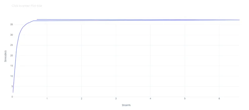
Fig:True stress vs strain of curve 2
2.The stress-strain data file obtained from the data digitizer software is opened in the excel to plot a graph between the true stress and true strain
as shown in the above fig.
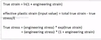
3.The true stress-strain data is then converted into effective plastic strain and stress to add to the material card. To keep the plot consistence, a cu
rve is fitted to the extracted data, and the data-points are taken from the curve. Using the following relation, the true stress-strain data is
converted into effective plastic stress-strain data:
Effective stress = true stress
Effective strain = Total true strain - elastic true strain
Effective strain = Total true strain - (true stress/Young's modulus)
4.The extracted data is to be set as a input curve and then recalled in the material model- MAT24.
5.From the plot it can be observed that there are some inconsistencies in the plot hence a curve is fitted to it using trend-line feature in excel. It
is made sure that the error is minimal. Given the nature of the graph, a logarithmic distribution gets a very close fit and hence is selected.
To match a suitable unit system, the units for stress were converted from KSI – Kilo pounds per square inch into GPa – Giga Pascal using following
conversions: 1 Kilo Pounds per square inch = 4.44822 KN = 6.8947572 Pascal.
To get good results we have make some equidistant spacing in the strain % so it will produce the curve which will result monotonically increasing
values.
| Strain % | True strain | Stress ksi | Stress gpa | True Strain | Eff stress | Eff plastic strain |
| 0.00851 | 0.0000851 | 1.87E+00 | 1.29E-02 | 1.0000851 | 1.29E-02 | -4.42E-06 |
| 0.0219 | 0.000219 | 4.67 | 3.22E-02 | 1.000219 | 0.0322 | -4.45E-06 |
| 0.028 | 0.00028 | 6.02 | 4.15E-02 | 1.00028 | 0.0415 | -8.04E-06 |
| 0.0425 | 0.000425 | 9.03 | 6.23E-02 | 1.000425 | 0.0623 | -7.06E-06 |
| 0.0474 | 0.000474 | 10.1 | 6.96E-02 | 1.000474 | 0.0697 | -9.25E-06 |
| 0.0559 | 0.000559 | 11.8 | 8.14E-02 | 1.000559 | 0.0814 | -5.59E-06 |
| 0.0632 | 0.000632 | 13.6 | 9.38E-02 | 1.000632 | 0.0938 | -1.87E-05 |
| 0.0681 | 0.000681 | 14.5 | 1.00E-01 | 1.000681 | 0.1 | -1.28E-05 |
| 0.0778 | 0.000778 | 16.5 | 1.14E-01 | 1.000778 | 0.114 | -1.15E-05 |
| 0.0887 | 0.000887 | 18.9 | 1.30E-01 | 1.000887 | 0.13 | -1.73E-05 |
| 0.0972 | 0.000972 | 2.06E+01 | 1.42E-01 | 1.000972 | 0.142 | -1.36E-05 |
| 0.108 | 0.00108 | 22.3 | 1.54E-01 | 1.00108 | 0.154 | 1.30E-05 |
| 0.126 | 0.00126 | 24.7 | 1.70E-01 | 1.00126 | 0.171 | 7.82E-05 |
| 0.146 | 0.00146 | 26.6 | 1.83E-01 | 1.00146 | 0.184 | 1.87E-04 |
| 0.166 | 0.00166 | 28.2 | 1.94E-01 | 1.00166 | 0.195 | 3.11E-04 |
| 0.19 | 0.0019 | 30 | 2.07E-01 | 1.0019 | 0.207 | 4.65E-04 |
| 0.222 | 0.00222 | 31.4 | 2.16E-01 | 1.00222 | 0.217 | 7.18E-04 |
| 0.256 | 0.00256 | 32.6 | 2.25E-01 | 1.00256 | 0.225 | 1.00E-03 |
| 0.3 | 0.003 | 33.7 | 2.32E-01 | 1.003 | 0.233 | 1.39E-03 |
| 0.351 | 0.00351 | 34.5 | 2.38E-01 | 1.00351 | 0.239 | 1.86E-03 |
| 0.398 | 0.00398 | 35.2 | 2.43E-01 | 1.00398 | 0.244 | 2.30E-03 |
| 0.45 | 0.0045 | 35.7 | 2.46E-01 | 1.0045 | 0.247 | 2.79E-03 |
| 0.499 | 0.00499 | 36 | 2.48E-01 | 1.00499 | 0.249 | 3.27E-03 |
| 0.558 | 0.00558 | 36.5 | 2.52E-01 | 1.00558 | 0.251 | 3.83E-03 |
| 0.601 | 0.00601 | 36.8 | 2.54E-01 | 1.00601 | 0.2513 | 4.25E-03 |
| 0.659 | 0.00659 | 37.2 | 2.56E-01 | 1.00659 | 0.2518 | 4.81E-03 |
| 0.7 | 0.007 | 37.4 | 2.58E-01 | 1.007 | 0.2522 | 5.21E-03 |
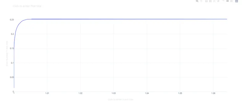
6.From the above graph we eliminating the linear deformation curve.So we have only non linear curve as shown.
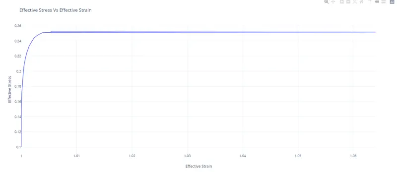
7.A dog bone specimen is given as a keyword file with having only the mesh and hence required cards are to be added by manually.
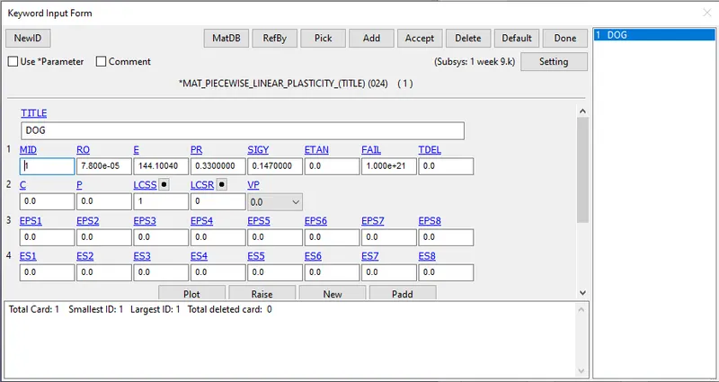
8.For the creation of cards firstly create a MAT_24_PIECEWISE_LINEAR_PLASTICITY for defining the behaviour of the elasto-plasic material.
By using this material it is very easy to consider the effect of rate of strain.
9.The values of both density and poisson's ratio is taken as default values.
The value of young's modulus is 20.9E+06 psi = 144.1004 GPa.
10.The curve LCID is assigned by using DEFINE_CURVE of effective stress versus effective strain.
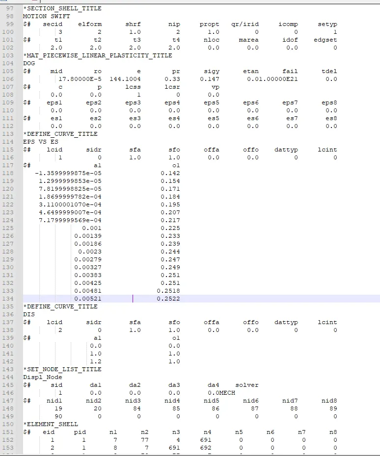
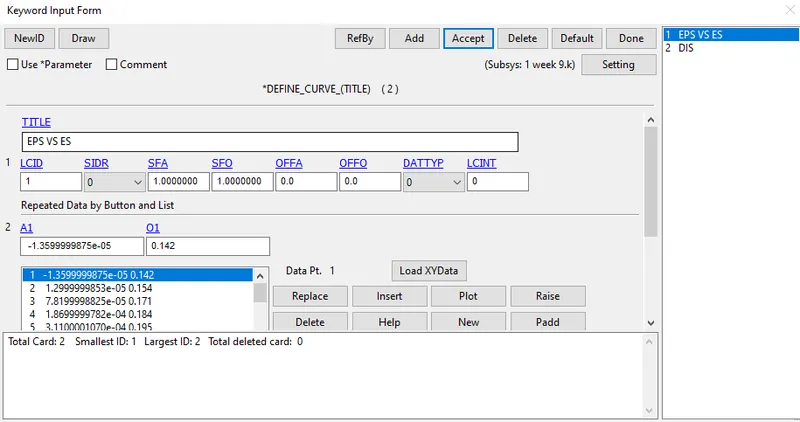
Fig: Engineering stress Vs Engineering Strain
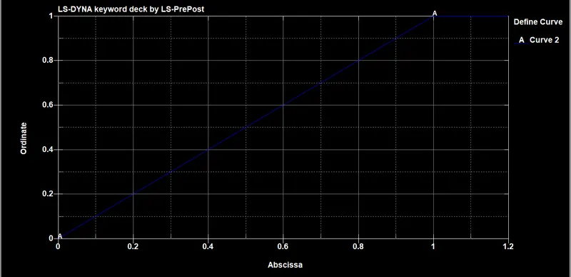
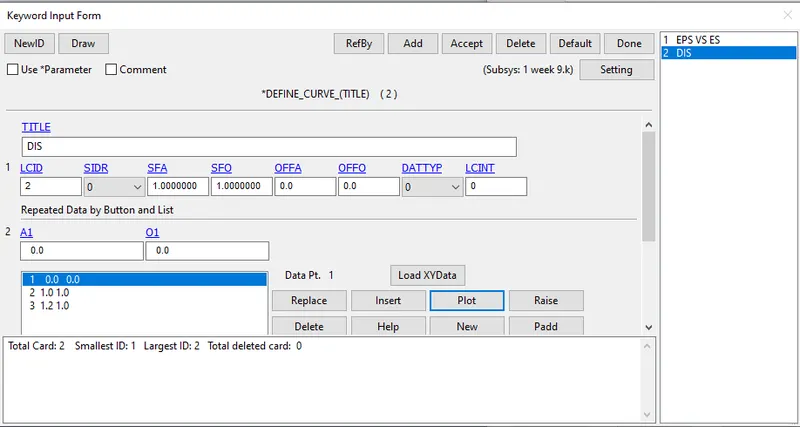
Fig:Displacement Curve
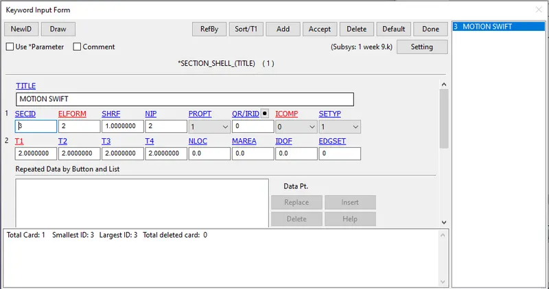
11.Creation of section shell card for assigning to the part as shown.
12.Create a material card as shown.
13.Now assign the both created material card and section shell card to the given dog bone part as shown in below fig.
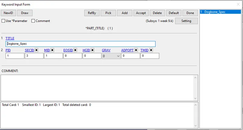
14.The nodes at the fixed end are constrained in X and Z direction only and Y direction is not constrained because of lateral expansion during
tensile test.
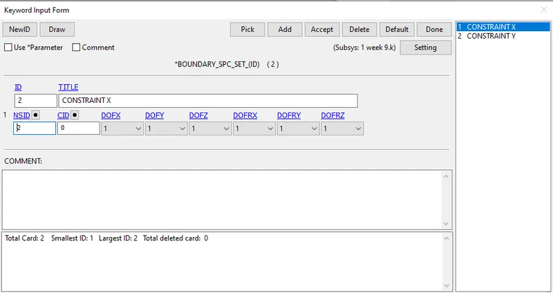
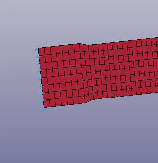
Fig:Constrain in x-direction
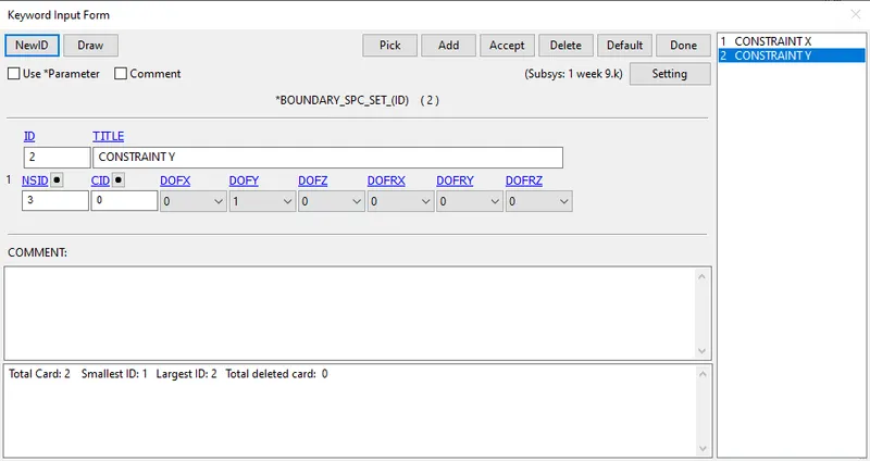
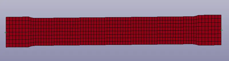
Fig:Constrain in y-direction
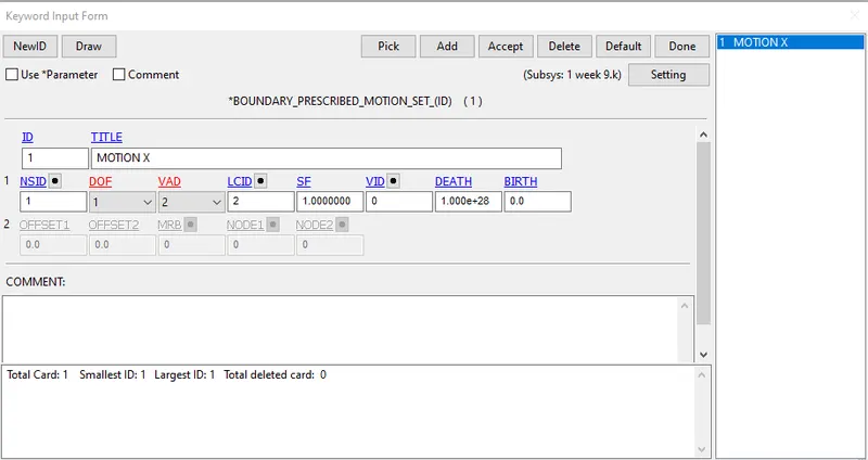
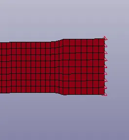
Fig:Boundary prescribed motion set
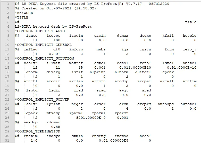
15.The time step value for the BINARY_D3PLOT and DATABASE_ASCII option for GLSAT and ELOUT is given as 0.01 ms.
DATABASE_EXTENT_BINARY card with STRFLG =1, is used to compute the elastic strain in the model.
Results And Discussion:
1.The animation of Von-Mises stress contour.
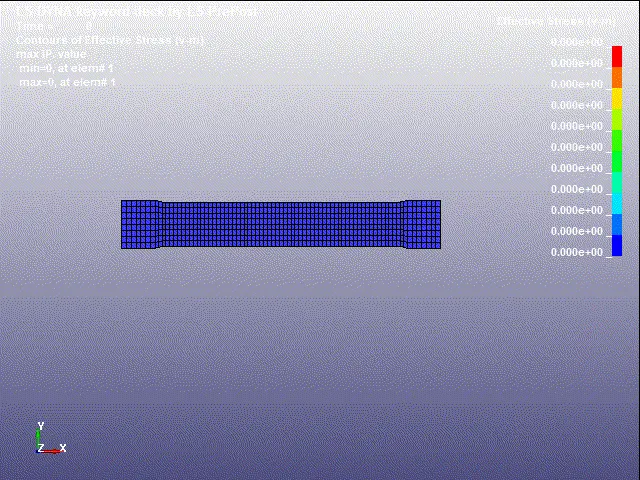
From the above animation of tensile test, the max von misses stressvalue is 0.2546 Gpa which is higher than the yield stress value of 0.1510 Gpa.
Therefore,the plastic deformation is occured in the specimen.The maximum stress is developed in the middle region of specimen but necking is not
observed till the end of simulation.
2.The animation of Effective plastic strain contour.
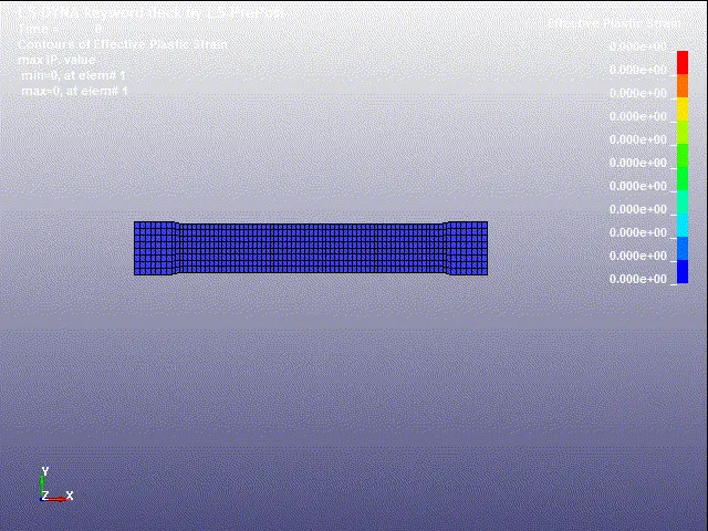
The max effective plastic strain from the above animation is very less 0.007651.Due to the presence of plastic strain the area of cross section of
specimen is going to be decreased at the middle.
3. X-Stress Plot:
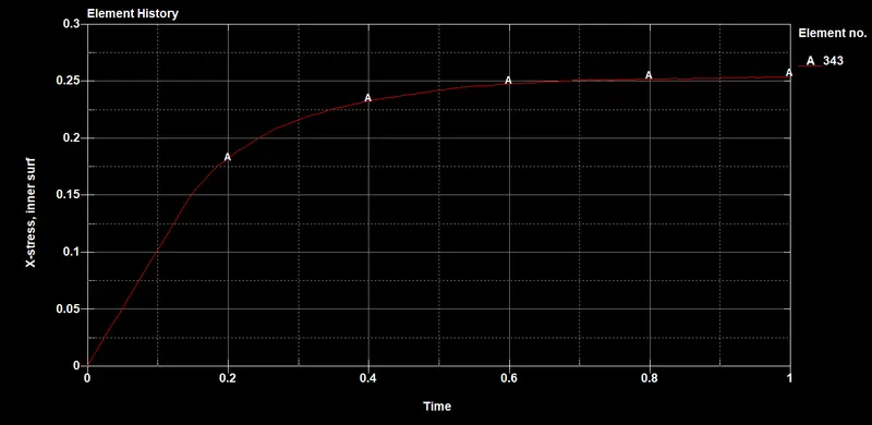
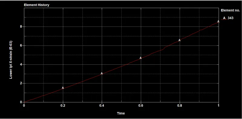
The true stress vs true strain plot obtained from simulation of tensile test on dog bone specimen is as shown in fig.13 which resembles the given
true stress vs true strain plot.
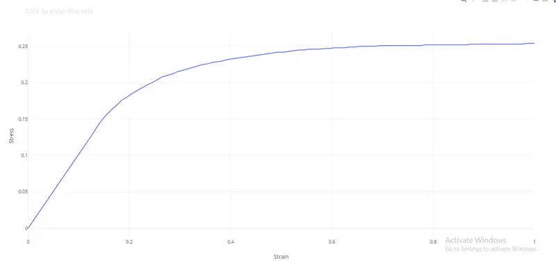
From the graph, the curve of raw true stress vs true strain plot exactly fits with simulation result curve of true stress vs true strain plot with dt0 =
0.0025. There is a deviation for simulation results with dt0 equal to 0.001 and 0.005 due poor convergence within the given initial time step size.
CONCLUSION:
1.The stress-strain data was extracted from the given diagram using data digitizer.
2.The extracted stress-strain data is used to model material using MAT_24 material card.
3.The material model is validated using tensile test on dog bone specimen by implicit analysis.
4.Learned to model material from raw data and validated it.