Week - 9 Material Modeling from Raw Data

Obejective:

To create material model with for MAT_24 PIECEWISE_LINEAR_PLASTICITY card from the given raw data using Data digitizer and LS-Dyna.

Procedure:

Case setup & Execution:

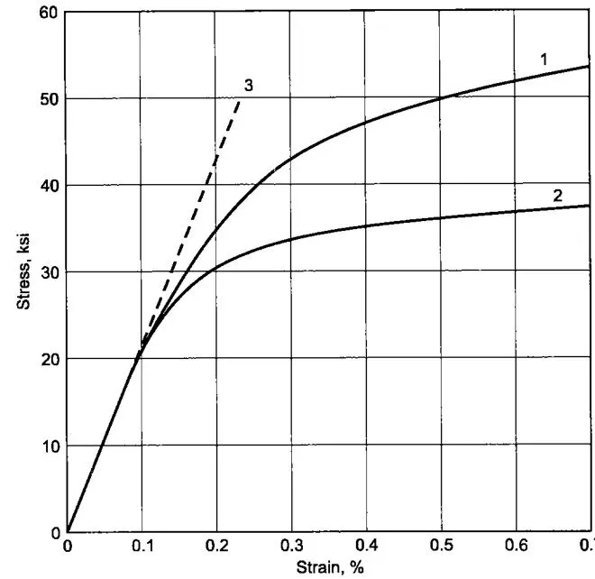
1. From the given image of material curve the data points are extracted using data digitizer

2. Then the extracted data is cleaned and plotted to check whether it is fitting to the original graph from the image.

\

From the image it can be understood that the stress value is in Ksi and the strain is percentage, so once the data is extracted we need to convert into the unit system that is followed here which is kg,mm,ms

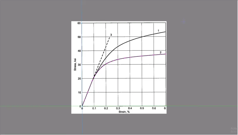
• The Data points to be extracted using Data digitizer is set with the values of x (0,0.7) and y (0,60)
• The second curve is captured here with the help of point capture option.
• The points which were extracted from the Data digitizer is imported into Excel sheet where it is cleaned to fit the original curve.

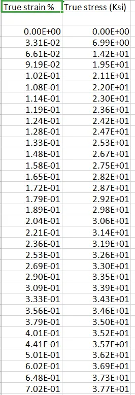
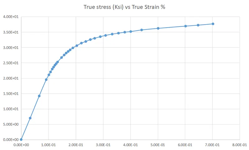
From the graph we can see that the extracted data graph is almost similar to the material curve image which we got, also we can notice that there is some noise in some areas which may be due to the human error happened while picking the points which should be cleaned before importing into the solver because LS-Dyna accepts only monotonically increasing curves.

Calculations:

• The stress values needed to be converted from Kilo pound per square inch (Ksi) to pascal
• The unit system used here is Kg,mm,ms so the convertion factor of Pascal to kg,mm,ms is `E^-09`
• So the stress value is multiplied with `E^-09`to get effective stress .
• As we already know that the value of stress is in ksi which is needed to be converted into kg,mm,ms and the strain values are in percentage which needed to be converted by dividing by 100

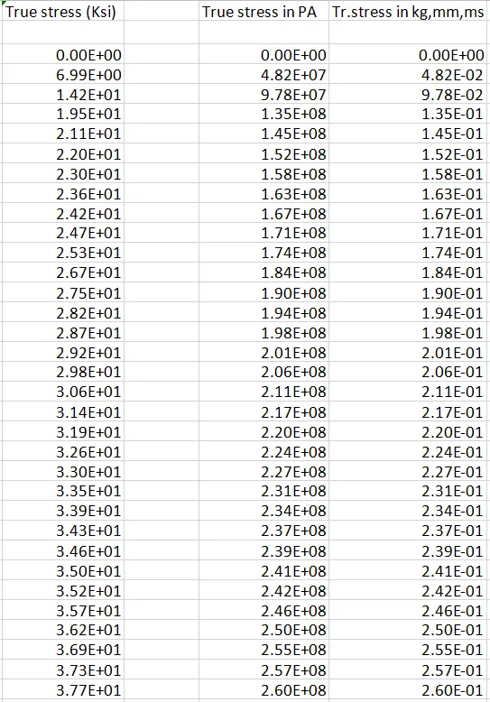
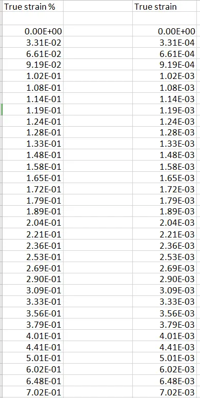
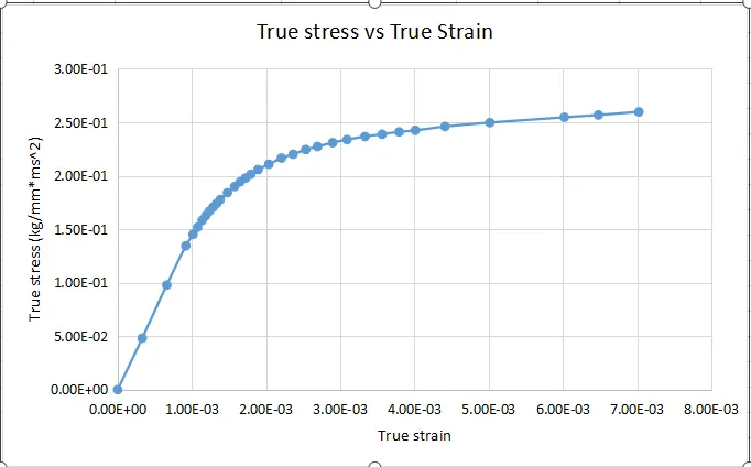
Now the value of youngs modulus is given as 20.9E+06 psi which needed to be converted into the unit system followed here i.e., kg,mm,ms

The SI unit of youngs modulus is Pa, so the given value needed to be converted into Pa first then it needed to be changed into the required unit system

For kg,mm,ms the factor to concert Pa to Kg,mm,ms is `10^-09`

`implies`Youngs modulus = 144.100 kg/mm*`ms^2`

For Effective plastic Strain:

The effective plastic strain can be calculated from the true stress and strain values to input the plastic region into the curve

• Elastic strain = True stress/Elastic modulus
• Effective plastic strain = (True strain - True stress)/Youngs modulus (E)

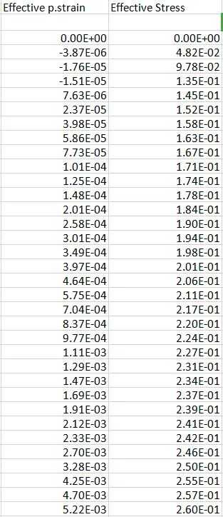
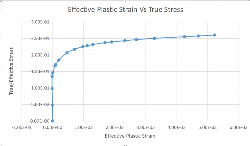
The Elastic region of the curve can be detrmined with the value of Density, Youngs modulus and poissons ratio, The plastic region can be obtained with the taking the yield point in the ablove graph

`implies` Siggy = 1.45E-01 gpa, this point is taken as the yield point and the curve beyond this is taken as Plastic region.

3. Importing the given tensile_test_mesh.k keyword file into LS-PP

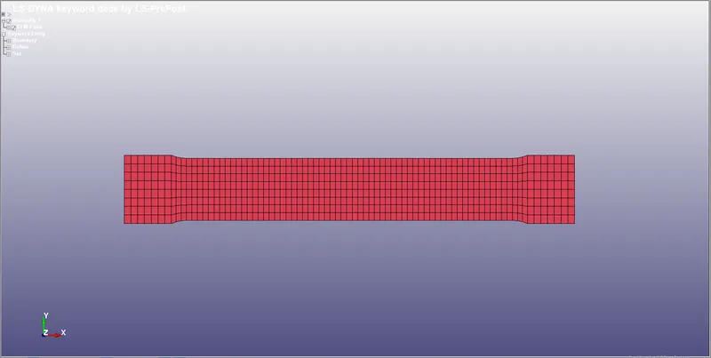
the file only consists of nodes and elements, other important keywords are needed to be defined.

4.Assigining Material and Section to part:

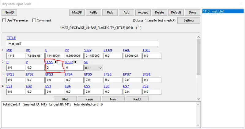
• For assigining the material the following steps are followed Keyword manager `rarr`All `rarr`Mat `rarr` Select the material card, here different material properties like mass density, youngs modulus, poisson's ratio and other recommended values are given
• Mat_24_Piecewise_Linear_Plasticity card with properties of steelassigned.

• Massdensity(RO)=7.800 e-06 kg/`mm^3`

• Young'sModus(E)=144.10 kg /`mm*ms^2`

• Poisson'sratio(PR)=0.3

• Yieldstress(SIGY)=0.145 kg /`mm*ms^2`

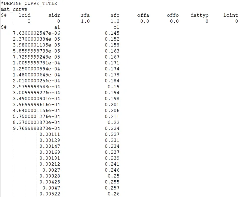
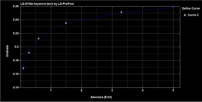
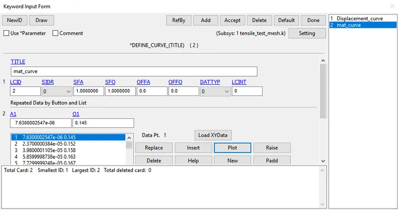
The values from the Effective plastic strain vs stress curve is taken and loaded as a curve to define the plastic region.

Section creation:

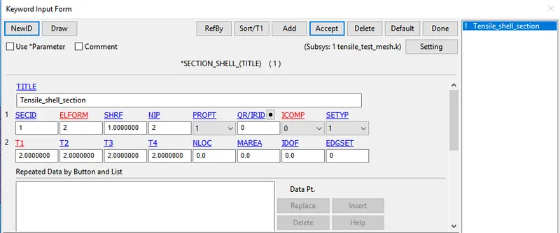
• Shell section is needed to be defined by selecting Keyword manager `rarr`All `rarr`Section `rarr`Shell
• Here the solid selection with element formulation 2 is defined with the thickness is given as 2 mm

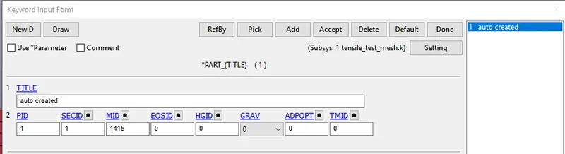
• For creating the part Keyword manager `rarr`model `rarr` part is used , then the respective section and material is assigned to it.

5. Boundary conditions:

For testing a model for tensile test, we need to fix one end and give diplacement to other end.

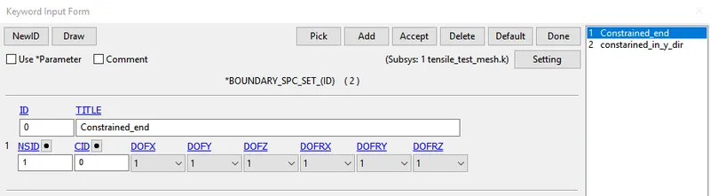
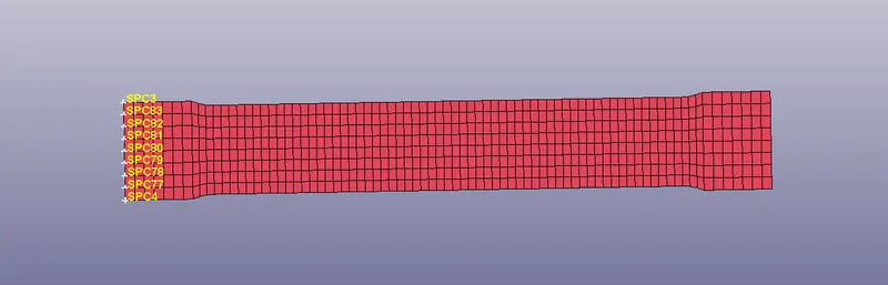
Creating SPC:

A Set of Spc is created at one end constraining all Dof's

Defining Prescribed motion set:

Node set is created at the opposite end in which the Spc is created by Create entity `rarr`Set nodes

In define curve keyword, we need to specify the displacement nodes by Define `rarr`Curve

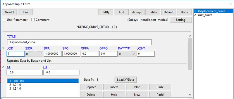
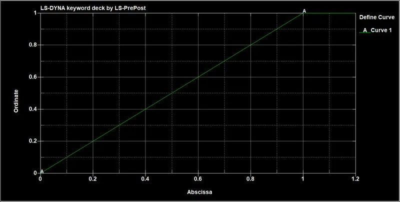
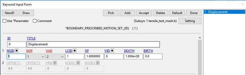
Here VAD is selected as two which refers to displacement.

6.Control Cards:

In LS prepost generally the solver used is Explicit, to perform in Implicit solver the following keywords are needed to be defined to switch from implicit to explicit

i.Keyword manager `rarr`All`rarr` control `rarr` Implicit_Auto

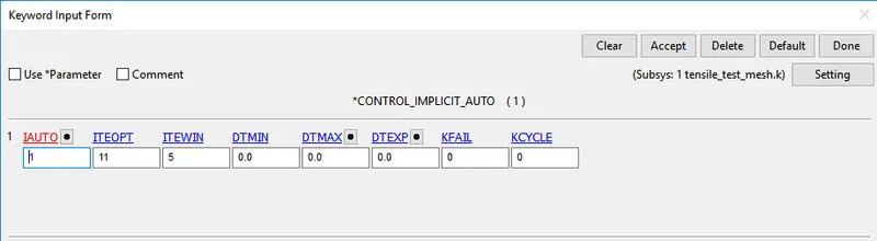
CONTROL_IMPLICIT_AUTO card is used for automatic time step control during implicit analysis. Input value for Automatic time step control flag = IAUTO = 1.

ii.Keyword manager `rarr`All`rarr` control `rarr` Implicit_General

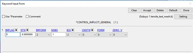
• CONTROL_IMPLICIT_GENERAL card is used to activate implicit analysis and define associated control parameters. This keyword is required for all implicit analyses.
• The input value for IMFLAG=Implicit/Explicit switching flag = 1 (implicit analysis)
• DT0=Initial time step size for implicit analysis = 0.005.

iii.Keyword manager `rarr`All`rarr` control `rarr` Implicit_Solution

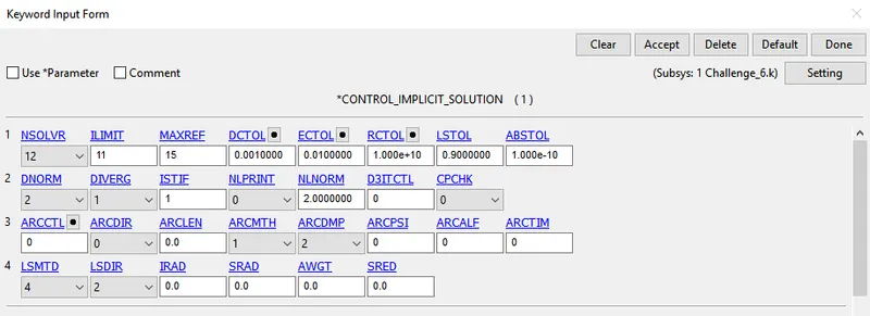
CONTROL_IMPLICIT_SOLUTION card is used to specify whether a linear or nonlinear solution is desired. The default values are set as it is in the card.

iv.Keyword manager `rarr`All`rarr` control `rarr` Implicit_Solver

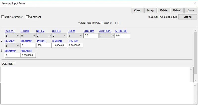
CONTROL_IMPLICIT_SOLVER card is used for implicit calculation.

v.Keyword manager `rarr`All`rarr` control `rarr` Termination

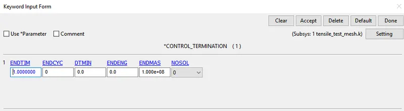
7. Output Request:

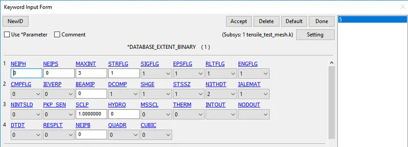
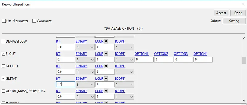
• Keyword Manager `rarr`Database `rarr` Extent_binary with STRFLG = 1 is given , this will compute the elastic strain in the model

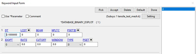
• Keyword Manager `rarr`Database `rarr` Binary D3plot `rarr` DT 0.1, this command prints the output at the end of each 0.01 ms

• Keyword manager `rarr`All`rarr` Database`rarr` ASCII_option from which GLSTAT,MATSUM and ELOUT option is selected with DT= 0.1 ms
• GLSTAT is defined with DT=0.01 ms which gives the output of energies such as Internal energies, kinetic energy & other types of energies

Run the simulation

• The keyword is saved in a separate folder and it is opened in Ls-Dyna manager

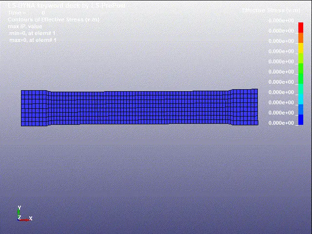
Effective stress:

Effective Strain:

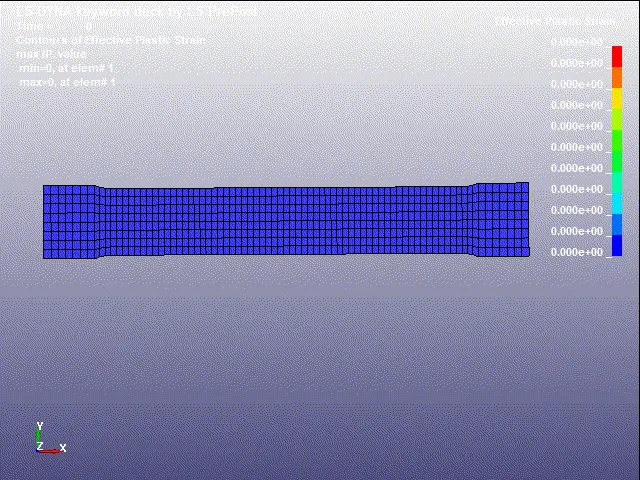
From the above plots it can be seen that the maximum stress observed is 0.2674 Gpa and maximum strain observed is 0.0073

Graph:

A Random element is taken at the middle and stress and strain graphs are plotted

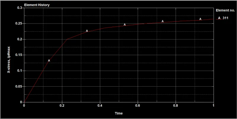
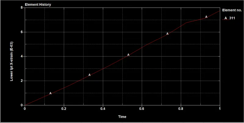
Stress Strain

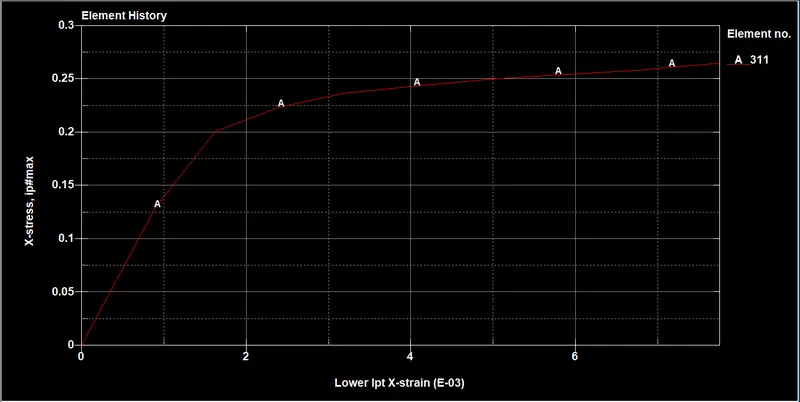
Stress vs Strain

Validation:

The from the above seen graph is imported into Excel sheet for validation purpose, which is done by corelating the graph which was plotted earlier between true stress and Strain.

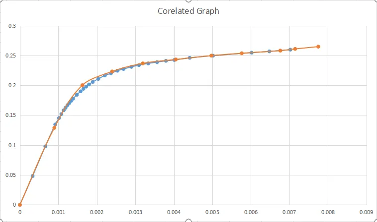
• Here we can see that there is an exact corelation between the experimental data and the raw data
• but due to some non linearities there is some deviation which is acceptable.

Conclusion:

From the given raw data image using Data digitizer material curve data is extracted and material model for MAT_24 PIECEWISE_LINEAR_PLASTICITY card is created and results are plotted then corelated with the raw data plot to be validated.