Week - 9 Material Modeling from Raw Data
Aim:-To create a material card from raw data and validate it.
Procedure:-
- First, they had given the graph of true stress and true strain graph.
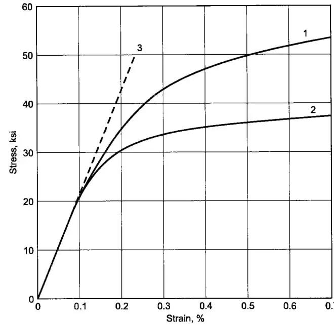
- By using this graph we need to convert the curve into x,y points
- By using get data graph digitizer software.
- First, we need to import the graph to the software.
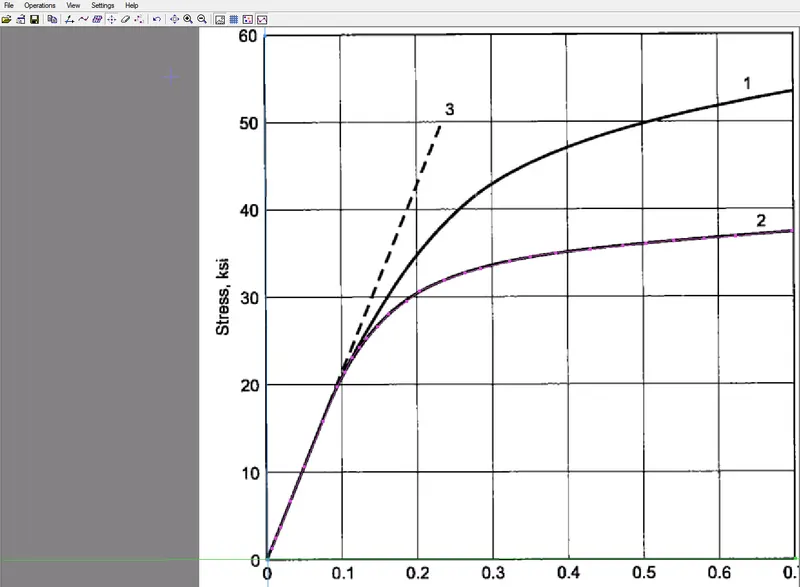
- Then we need to select a set scale from the menubar and the set minimum and maximum value of x,y.
- Then select point capture mode and trace the graph then we can see the x,y values are been plotted.
- Select file and select save data.
- We need to convert it into unit system of Kg mm ms.
1ksi=6.84810^-3 N/mm^2
- In the material model, we need to import the graph as effective plastic strain vs effective stress(true stress).
- To calculate effective plastic strain
effective plastic strain=true strain-true stress/E
Where E = Young's modulus(given E=20.9E+06 psi)
Convert psi to N/mm^2
1psi=144.1 N/mm^2
| TRUE STRAIN% | TRUE STRESS ksi | TRUE STRAIN | TRUE STRESS | EFFECTIVE PLASTIC STRAIN |
| 0 | 0 | 0 | 0 | 0 |
| 6.10E-03 | 1.25E+00 | 6.09934E-05 | 0.008611243 | 1.23463E-06 |
| 1.10E-02 | 2.39E+00 | 0.000109876 | 0.016505603 | -4.66668E-06 |
| 1.71E-02 | 3.64E+00 | 0.000170869 | 0.025116846 | -3.43204E-06 |
| 3.05E-02 | 6.66E+00 | 0.000305218 | 0.045928688 | -1.35097E-05 |
| 4.88E-02 | 1.06E+01 | 0.000488324 | 0.073198653 | -1.96473E-05 |
| 7.44E-02 | 1.58E+01 | 0.000744471 | 0.109078625 | -1.24935E-05 |
| 9.28E-02 | 1.98E+01 | 0.000927577 | 0.136348591 | -1.86311E-05 |
| 1.04E-01 | 2.14E+01 | 0.001037014 | 0.147827363 | 1.11473E-05 |
| 1.13E-01 | 2.31E+01 | 0.001134402 | 0.159307372 | 2.8869E-05 |
| 1.23E-01 | 2.43E+01 | 0.001231477 | 0.167196789 | 7.11944E-05 |
| 1.33E-01 | 2.53E+01 | 0.00132849 | 0.174368086 | 0.00011844 |
| 1.47E-01 | 2.66E+01 | 0.001473882 | 0.183688795 | 0.000199151 |
| 1.62E-01 | 2.81E+01 | 0.001619338 | 0.193727623 | 0.000274941 |
| 1.86E-01 | 2.96E+01 | 0.001861178 | 0.203756563 | 0.000447184 |
| 2.03E-01 | 3.07E+01 | 0.002030542 | 0.211638563 | 0.000561849 |
| 2.36E-01 | 3.19E+01 | 0.002356593 | 0.220222614 | 0.00082833 |
| 2.63E-01 | 3.28E+01 | 0.002634201 | 0.225939134 | 0.001066268 |
| 2.84E-01 | 3.33E+01 | 0.002839332 | 0.229508715 | 0.001246628 |
| 3.23E-01 | 3.41E+01 | 0.003225373 | 0.235214111 | 0.001593075 |
| 3.50E-01 | 3.46E+01 | 0.003502792 | 0.238776276 | 0.001845775 |
| 3.84E-01 | 3.50E+01 | 0.00384039 | 0.241614142 | 0.002163678 |
| 4.30E-01 | 3.55E+01 | 0.004298468 | 0.244439648 | 0.002602148 |
| 4.73E-01 | 3.59E+01 | 0.00473245 | 0.247267626 | 0.003016505 |
| 5.03E-01 | 3.62E+01 | 0.00503384 | 0.249391082 | 0.00330316 |
| 5.41E-01 | 3.65E+01 | 0.005407519 | 0.251507121 | 0.003662154 |
| 5.81E-01 | 3.67E+01 | 0.005805232 | 0.25290257 | 0.004050183 |
| 6.23E-01 | 3.70E+01 | 0.006227103 | 0.255013666 | 0.004457404 |
| 6.97E-01 | 3.76E+01 | 0.006974461 | 0.259245745 | 0.005175392 |
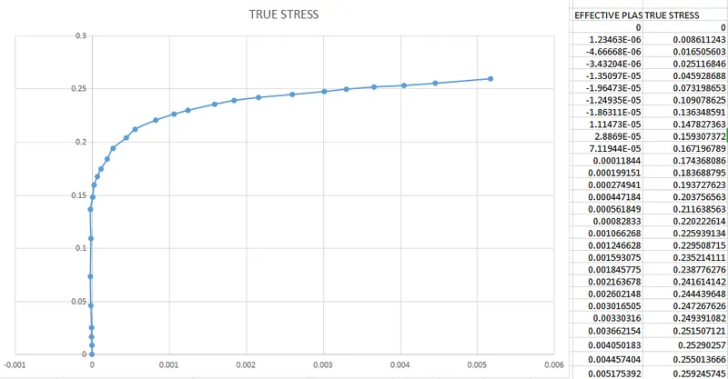
- To import the model the will be considered from the Yield stress.
- After the calculations, we need to open the ls pre-post with the given model.
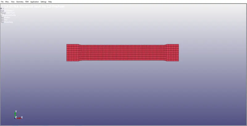
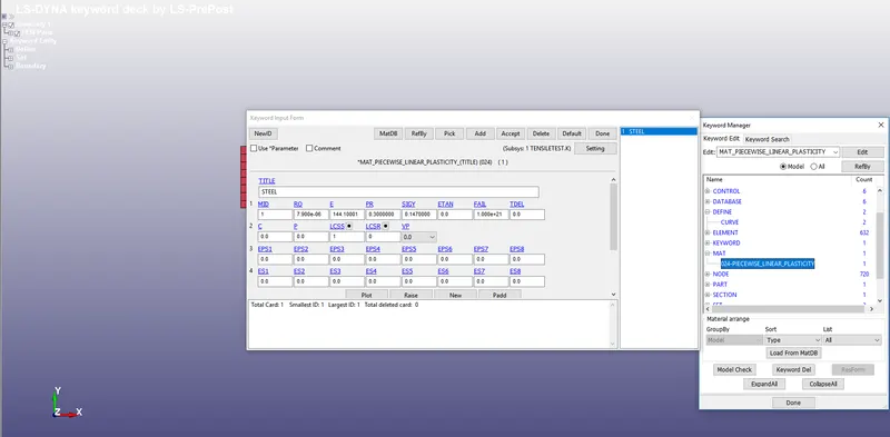
- Then we need to go to keyword and select MAT 24(PIECE WISE LINEAR PLASTICITY)
- We will property of steel in kg mm ms
- Where we will consider the yield stress value after the linear slope.
E=144.100,SIG_Y=0.147.
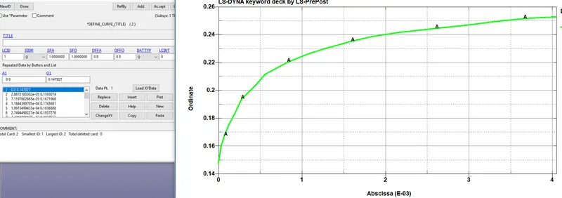
- Before we need to define the curve.
- To define the curve we need to go to define and give the values of the material.
| EFFECTIVE PLASTIC STRAIN | TRUE STRESS |
| 0 | 0.147827363 |
| 2.8869E-05 | 0.159307372 |
| 7.11944E-05 | 0.167196789 |
| 0.00011844 | 0.174368086 |
| 0.000199151 | 0.183688795 |
| 0.000274941 | 0.193727623 |
| 0.000447184 | 0.203756563 |
| 0.000561849 | 0.211638563 |
| 0.00082833 | 0.220222614 |
| 0.001066268 | 0.225939134 |
| 0.001246628 | 0.229508715 |
| 0.001593075 | 0.235214111 |
| 0.001845775 | 0.238776276 |
| 0.002163678 | 0.241614142 |
| 0.002602148 | 0.244439648 |
| 0.003016505 | 0.247267626 |
| 0.00330316 | 0.249391082 |
| 0.003662154 | 0.251507121 |
| 0.004050183 | 0.25290257 |
| 0.004457404 | 0.255013666 |
| 0.005175392 | 0.259245745 |
- After creating the material we need to create the section .
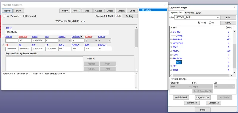
- Here we selected the section as 16 as fully integrated and thickness as 2mm.
- After creating the material and section we need to combine to part.
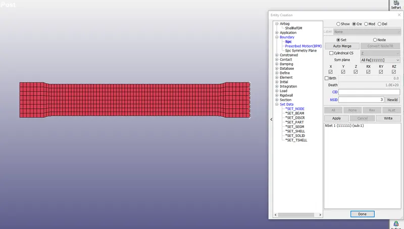
- Then we need boundary conditions like fixing the one end and another end we need to give the curve of displacement.
- To make constrained select create entity and select boundary conditions and select SPC and lock all directions.
- From prescribed motion, we need to provide displacement vs time graph.
- To define go to define and input the x,y values and save it.
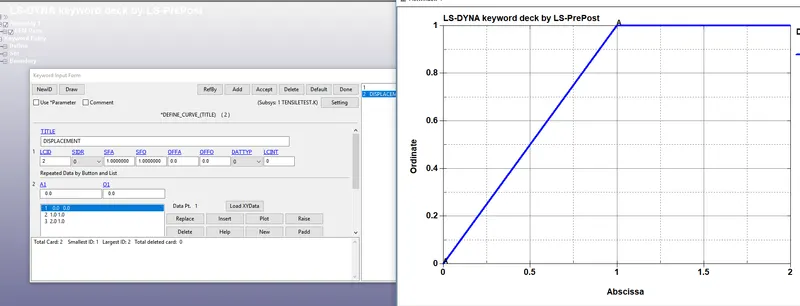
- Go to prescribed motion set and make node as set and import the curve and give VAD=2 and save it.
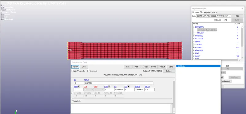
- For this simulation, we are going to use only the implicit solver.
- To activate the implicit solver we need to select control implicitly and select IMFLAG as 1.
- The solver will be activated and we can give the initial time step to start.
- Here we had given the initial time step as 0.01ms.
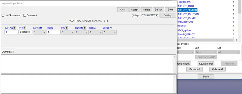
- And we need to activate the auto time step to increase the chance of convergence.
- And also we can constrain the number of iteration to be solved.
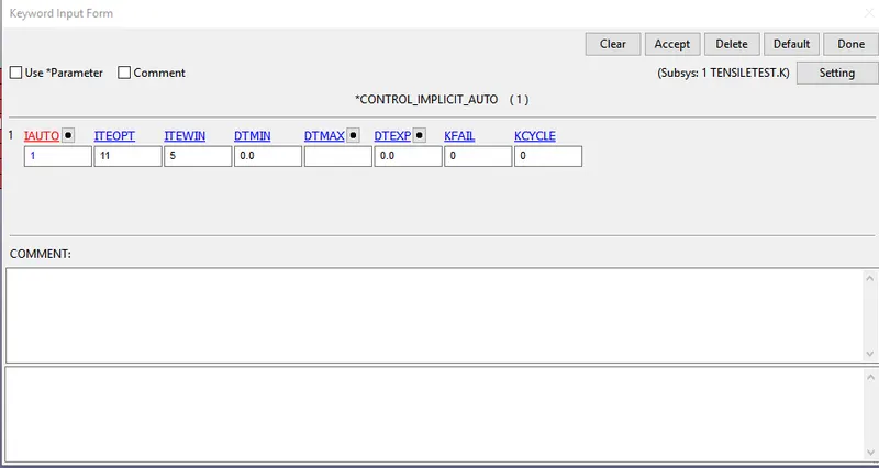
ITEOPT: Optimum equilibrium iteration count per time step.
ITEWIN: Allowable iteration window. If iteration count is within ITEWIN
iterations of ITEOPT, the step size will not be adjusted for the next
step.
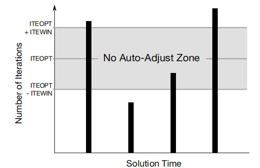
- For a certain time step if the solver is converging in less number of the steps then the time step will automatically increase.
- If it is unable to solve for that time step it will increase the iterations.
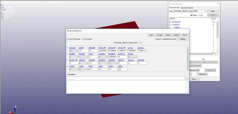
- CONTROL_IMPLICIT_SOLUTION:-These optional cards apply to implicit calculations. Use these cards to specify whether a linear or nonlinear solution is desired.
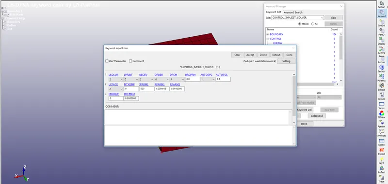
- CONTROL_IMPLICIT_SOLVER:-These optional cards apply to implicit calculations. The linear equation solver performs the CPU-intensive stiffness matrix solution.
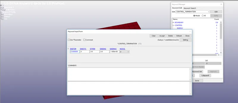
- We need to give the end termination time to solve.
- We need to give output requests to get results from the post-processor.
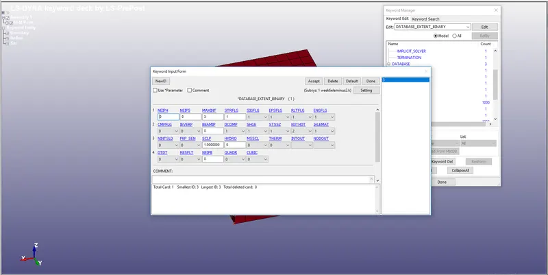
- This is used to get the strain result from the elements STRFLG=1.
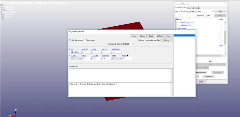
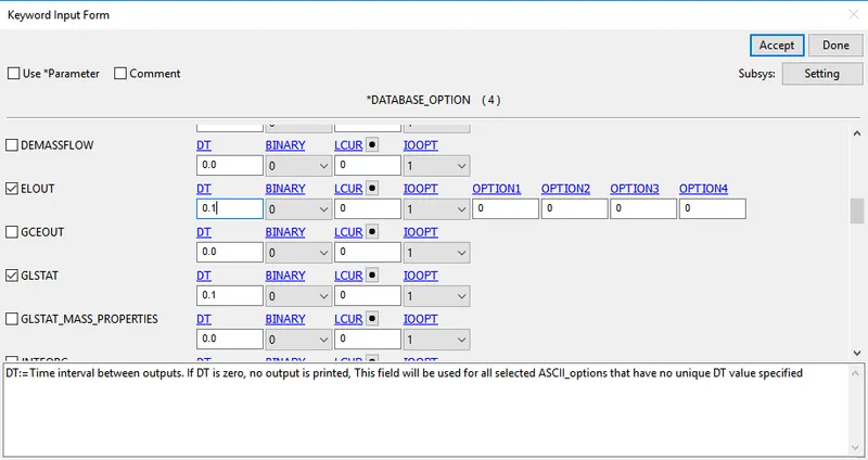
- And we need to give access to binary d3plot and In ASCII glstat.
Results:-
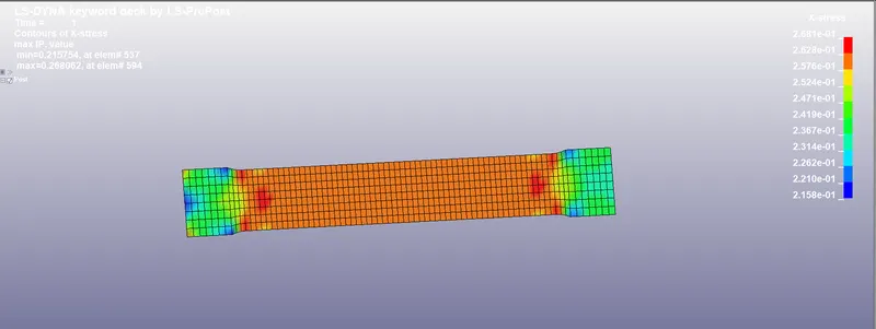
- Here the maximum stress attained by the model is 2.681e-01 N/mm^2
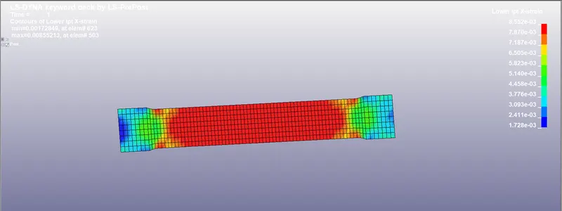
- The maximum strain attained by the component is 8.552e-03
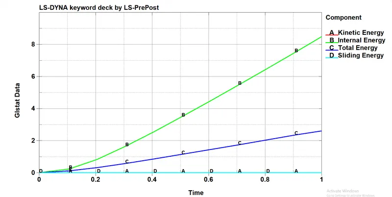
- Where here kinetic energy is neutral because there is very little displacement so that the kinetic energy is constant.
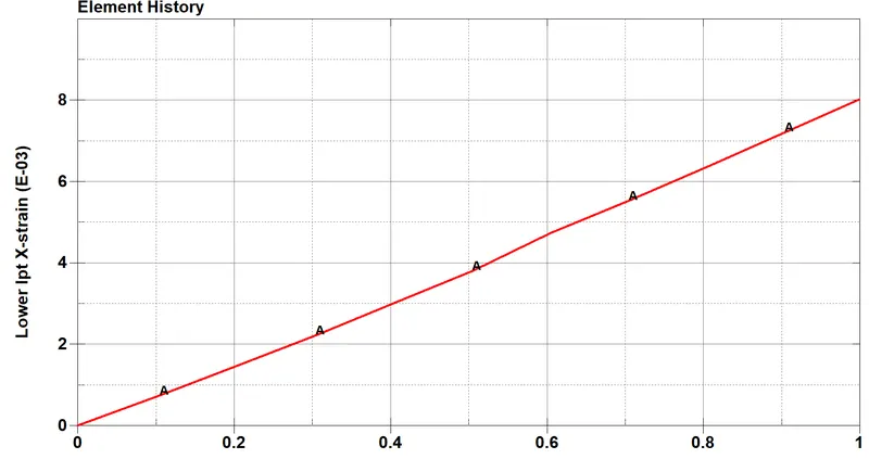
- Here we are going to plot a graph of x-strain and x- stress which is true stress vs true strain.
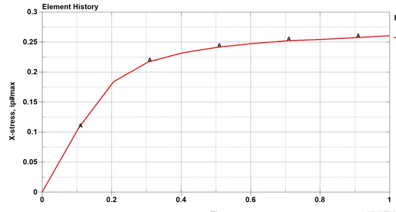
- Now we need to cross plot the above two graphs.
- To cross plot we need to save the two files and the go-to post-processing then select xy plot
- Then load the file and cross plot the graph.
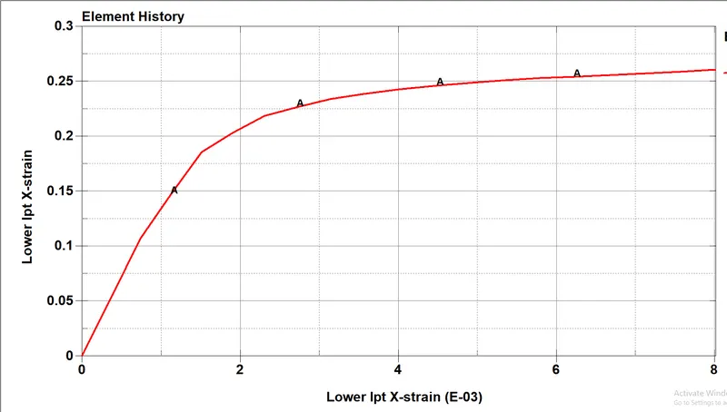
- Now we need to correlate the material data and graph after stimulating.
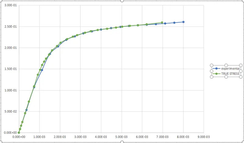
- There is an exact correlation between the material data and experimental data.
- But due to some nonlinearities, the is some deviation this is accepted.
CONCLUSION:-
- Understood how to extract material curve data from the experimental value.
- Understood how to import material curve to the material card in the solver.
- Understood how to correlate the experimental data with material curve data.