Week - 9 Material Modeling from Raw Data
AIM:
To use the given true stress-strain curve of graphite iron casting and develop the material card using either MAT_024 or MAT-018 in lsdyna. Then simulate the dog bone specimen and compare the stress-strain curve obtained from simulation result to the actual stress-strain curve.
SOLUTION:
The below shown image is the given true stress-strain curve of graphite iron.
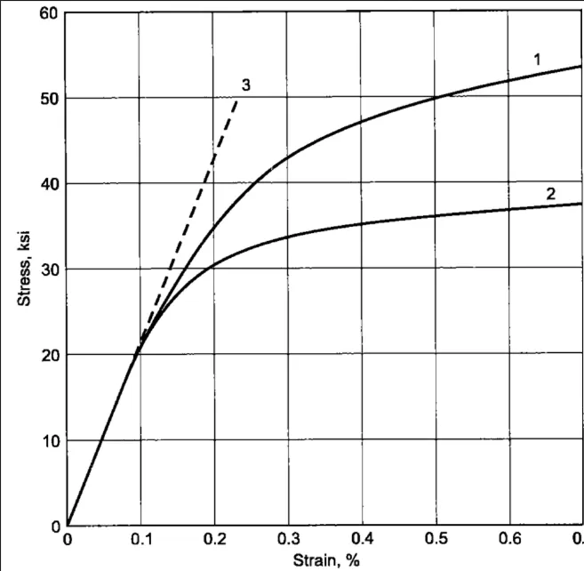
Youngs modulus of given graphite iron casting = 20.9E+06 psi.
The unit system kg/mm/ms is being followed thought out the simulation.
STEP:1
Digitizing the image and extracting x,y points of the selected curve (Curve number 2 is selected).
- Open Originpro and import the image of stress strain curve.
- Click digitize image, select the autotrace line by points option and click on the curve and it will create points over the curve as shown below.
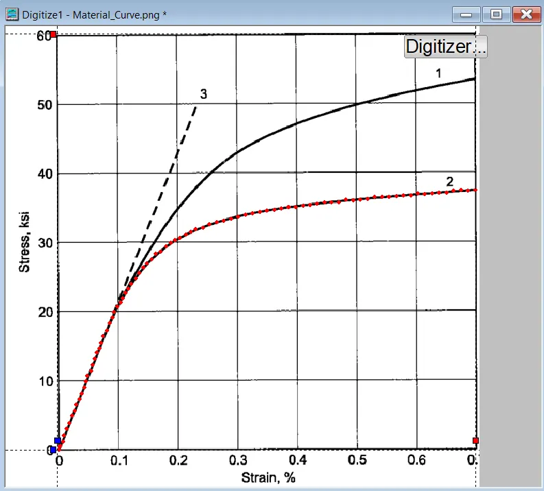
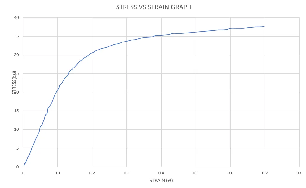
- Now export the extracted x,y plots as a xls format and open it in microsoft exel.
STEP:2
CURVE FITTING:
- As the extracted curve from the digitizer is having noise we have to do curve fitting. So curve fitting helps to find the best fit for sets of data points.
- For curve fitting open matlab>go to apps>click on curve fitting.
- Import the x,y plots of the curve into matlab. In the curve fitting tool, select the x data as strain plots and y data as stress plots and select the curve fitting method as smoothing spline. with Smoothing parameter 0.9959886 the best fit for the curve is achieved.
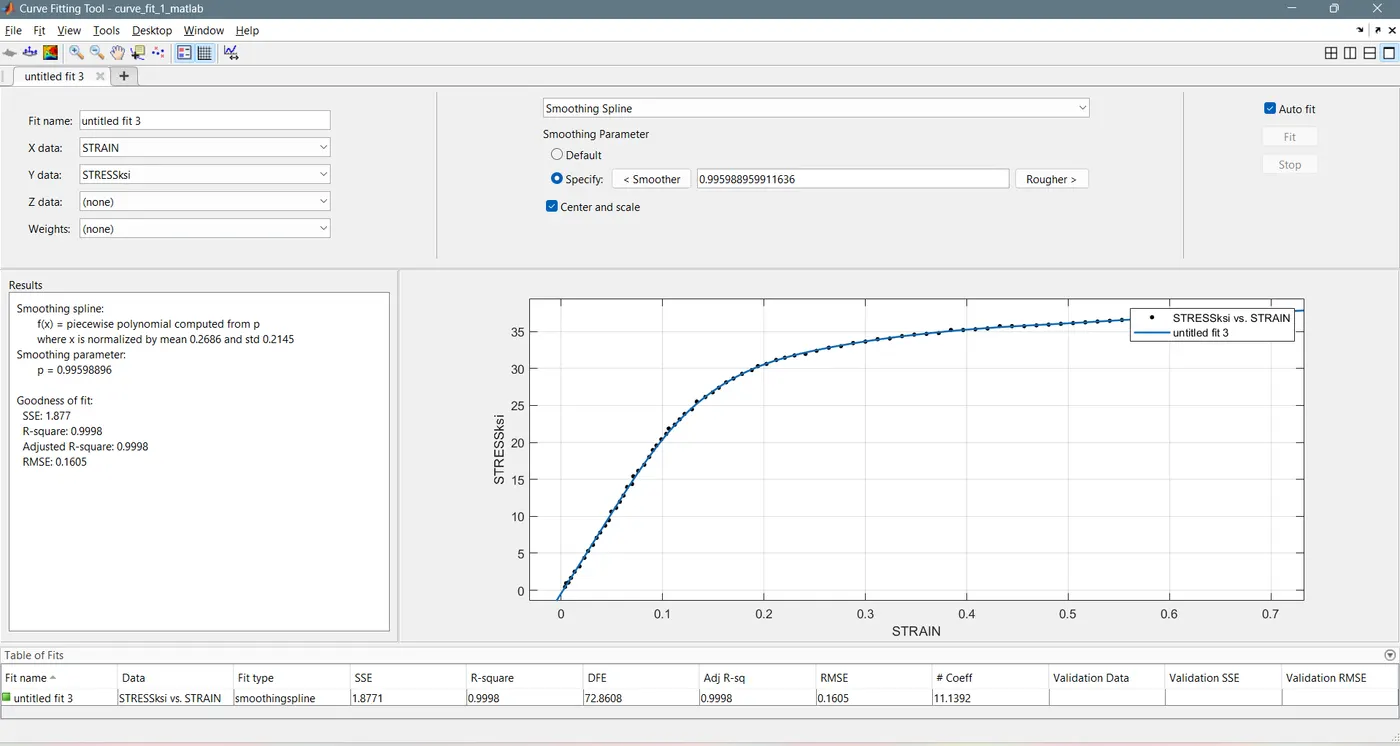
- Now generate the code. Now edit the code and run it.
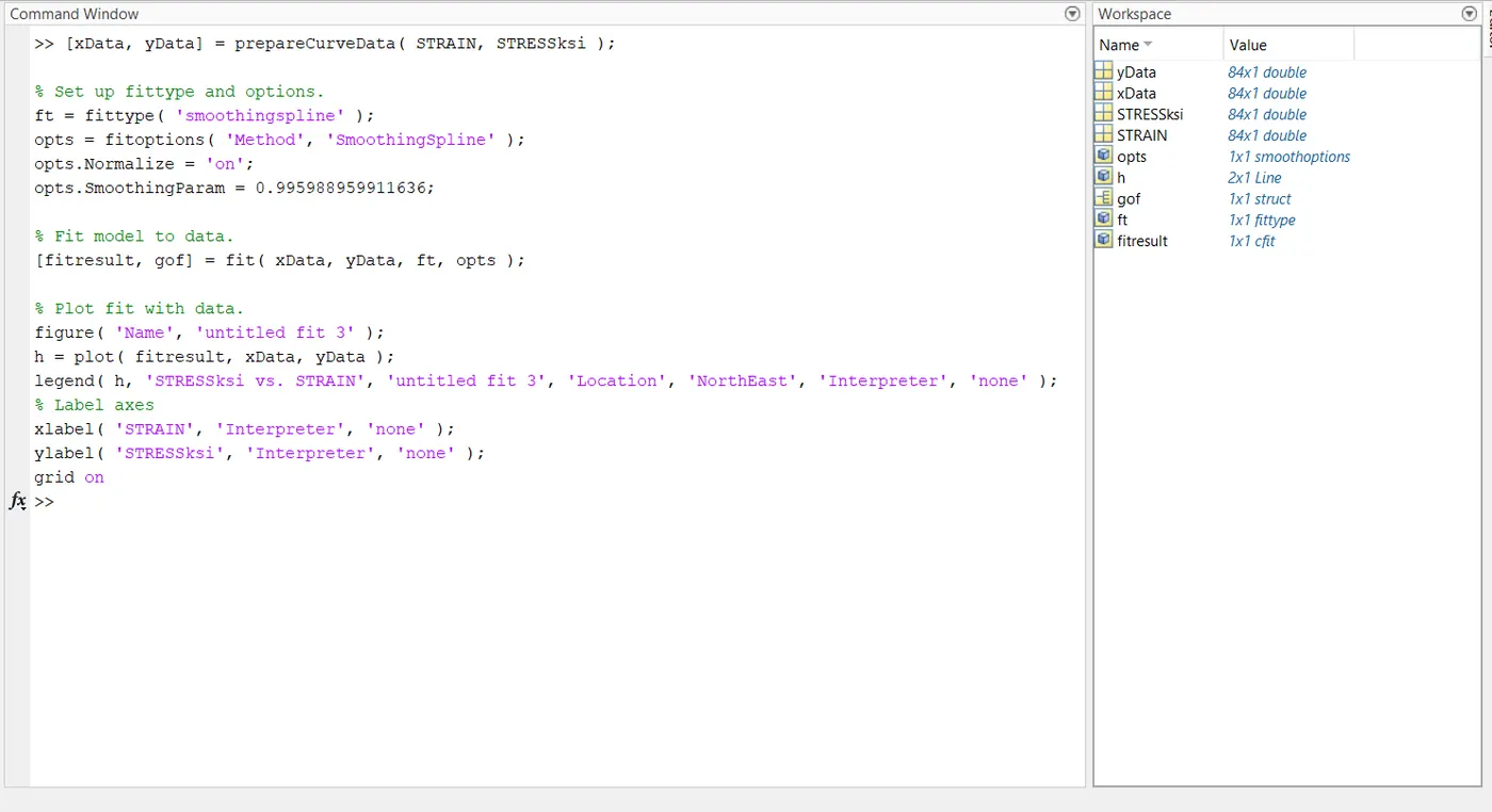
- It will create a cfit object. Use it to create an fitted x,y plots as shown below.
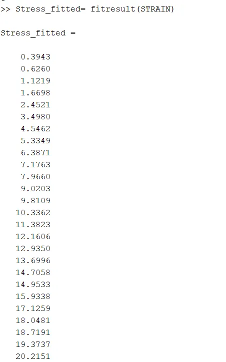
- Now copy this fitted data points to the exel file and plot it.
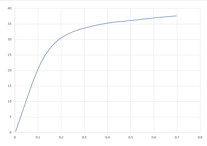
STEP:3
Unit conversion:
- To convert the stress from ksi to kg/(mm.ms2) we have to multiply with 0.006895
- To convert the strain from percent we have to divide by 100.
- Use the exel formula option and apply to all the values in the respective columns.
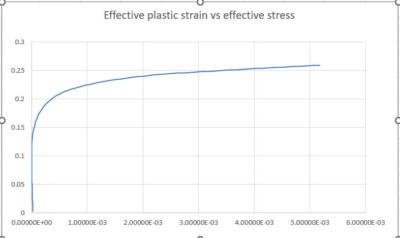
- Now the fitted stress strain curve is obtained with required unit and it is a true stress vs true strain curve. For mat 024 material card, the load curve should be defined in effective plastic strain vs effective stress curve. For that, use the below formula.
- Effective stress= True stress
- Effective plastic strain= True strain-(True stress/E).
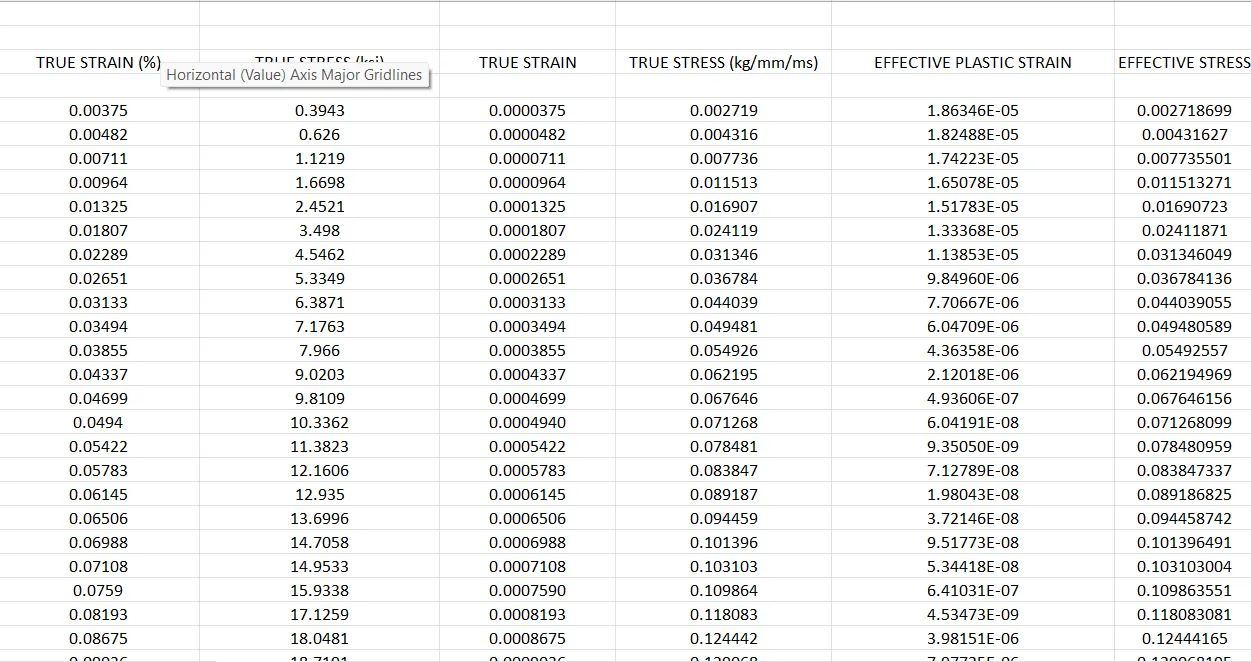
- Effective plastic strain vs effective stress curve obtained as shown below.
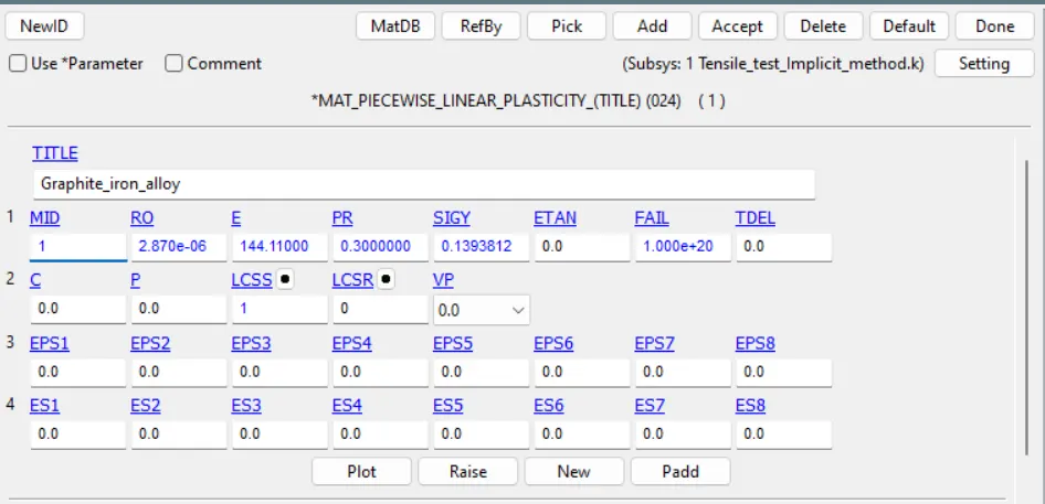
- youngs modulus=20.9E+06 psi, After unit converstion it is 144.11 kg/(mm.ms2)
- Density = 2.87e-06 kg/mm3
- Yield stress is found out by drawing line at 2% of strain and it is found out as 0.13938115 kg/(mm.ms2)
- Length of the bar = 145mm
- Displacement given to the bar = 3.5mm
STEP :4
- Now open the dog bone specimen key file in ls prepost and now first we have the load the effective plastic strain vs effective stress curve. First define a curve with 0,0 and save the keyword and open it in the notepad++. There you can copy and paste the x,y plots from exel to notepad++ and save the file and reopen the file in ls prepost.
- Now the Curve is starting with values which are nearly equal to zero so those x,y points are negleted and the updated curve is as shown below.
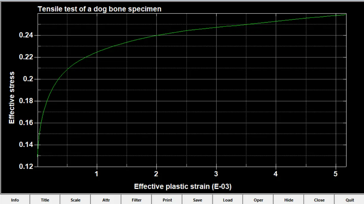
- Now Go to lsprepost>keywork>mat>024_piecewise_linear_plasticity and enter the details as shown below.
- Now open the section>shell>Elform as 16>thickness as 6mm.
- Now go to Part>select the secid>mid accordingly.
STEP 5:
APPLYING BOUNDARY CONDITIONS:
- The tensile test is done as the one of the specimen is fixed and the other is applied a load. A gauge is fitted between the specimen and it will show the displacement of the specimen for the particular load applied.
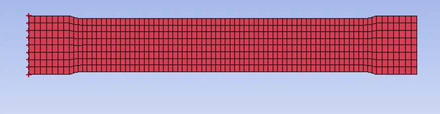
- Here First the mid nodes of both the sides of the specimen should have constrained only in y translation and it is free to move in x and z direction.
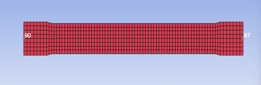
- And the all the nodes of one end is constrained in all the direction except y translation.
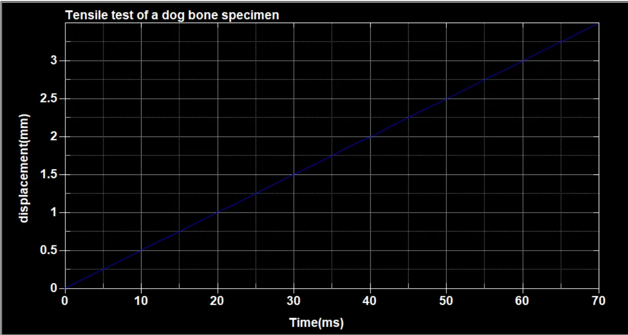
- Now define a load curve to define the displacement that is being applied at the other end as shown below.
- In the other end create and node set and go to Boundary>Prescribed_motion_set>Select the dof as x translational. Pick the load curve and ok.
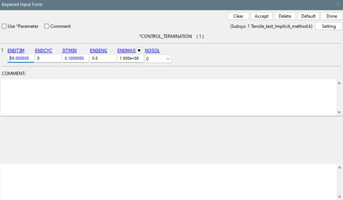
- Now go to control termination>since the displacement curve is defined up to 71ms we given end time as 70ms.
- Since the problem is non linear, implicit solver is used. go to control>implicit auto>Enter minimum time step as 0.001. If the system goes below 0.001 time step it will terminate.
- Now control> Implicit general>IMFLAG value as 1 for implicit solver>Remaining kept as default.
- Control> implicit solutions> NSOLVER as 12> remaining kept as default.
- control>implicit solver>Select print output summary and warning>remaining kept as default.
- Now data base Binary d3plot>ASCII OPTIONS> ELOUT>NODOUT>GLSTAT.
- Create history nodes and elements.
- Run the key file in ls dyna.
STEP:6
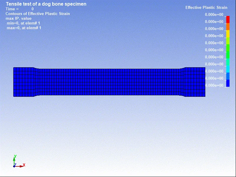
EFFECTIVE PLASTIC STRAIN CONTOUR:
EFFECTIVE STRESS CONTOUR:
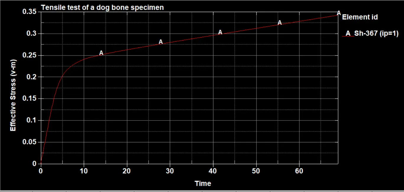
Curve of Effective stress obtained from the simulation:
Curve of Nodal displacement obtained from the simulation:
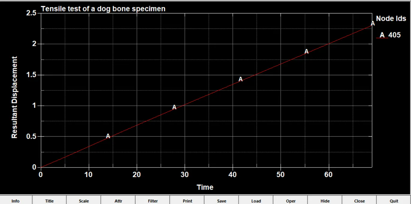
Save this curves as x_Y pairs and import it to ls dyna. Now from the resultant displacement, strain value is calculated and thus the true stress strain curve has been extracted from the simulation.
STEP:7
Comparison of simulation and actual result.
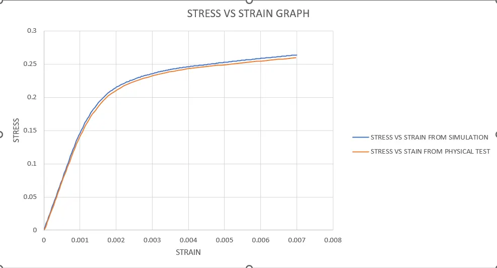
From the simulation curve up to elastic limit the equation is obtained as,
0.050486x - 0.000369y = 0
From the above equation the value of youngs modulus can be determined as.
E=136.82 kg/mm.ms2
The actual value of youngs modulus is E = 144.11 kg/mm.ms2
The percentage difference = ((144.11-136.82)/144.11)*100
= 5.0586%
The percentage in youngs modulus obtained from simulation has 5.0586% from the actual value.
CONCLUSION:
Thus from the given true stress vs true strain curve, the curve had been obtained in x,y plots using data digitizer. Using this, a material card had been developed and it was analized through a tensile test of a dog bone specimen. Finally the simulation and actual result had been compared and it is found that there is 5.0586�viation in simulation from the actual which is acceptable.