Week - 9 Material Modeling from Raw Data

Material Modeling From Raw Data

Objective

• Create a MAT024 material card from raw data
• Validate the material card using a uniaxial test simulation

Procedure

The first step into creating a MAT024 material card is to obtain the stress-strain data from a uniaxial test of a material, graphite iron casting in this case, described in the following figure:

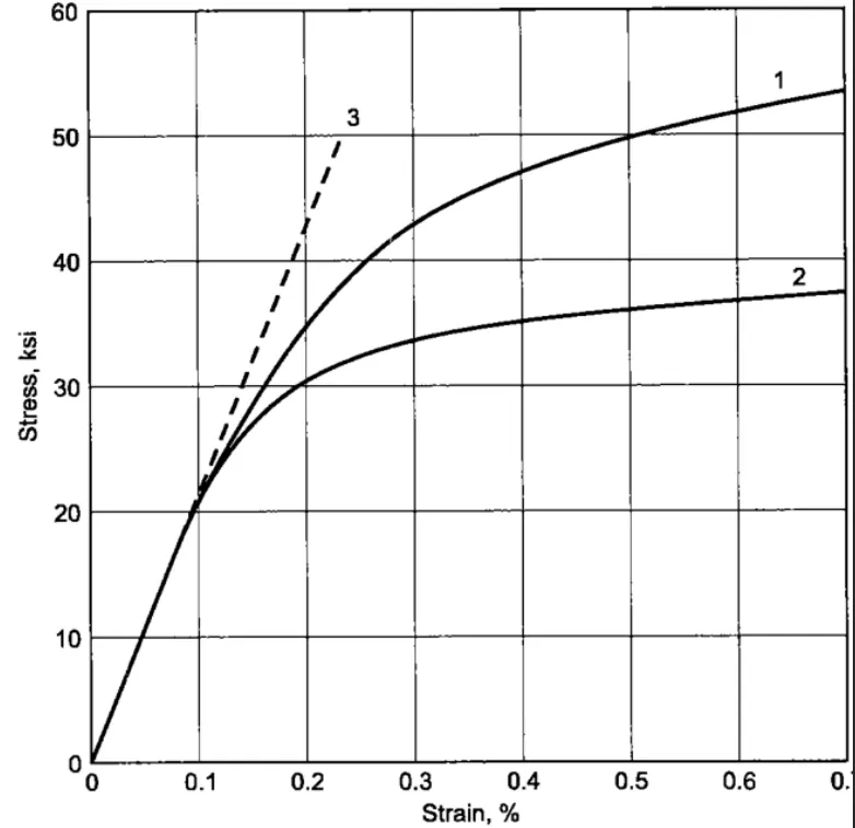
To obtain the data for the line 2, we will use an external software (such as MATLAB or Origin) to interpolate the data points. Regardless of the software used, the following steps must be completed:

• Load the graph into the software

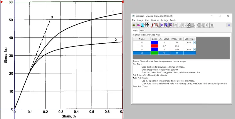
• Define two points in the X and Y axis to interpolate the data

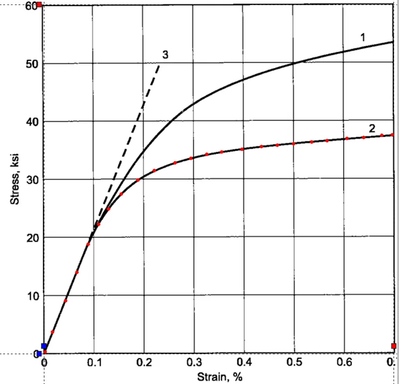
• Manually select the curve of interest by picking multiple points

• Export the data and plot again to verify results

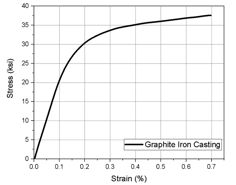
By using Hooke's Law in the points between 0.015% and 0.09% strain we can average a Young's Modulus

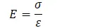
• Note: Strain values are given in terms of %, meaning they should be divided over 100 for the real strain value

The next step is to convert all the extracted data points into the Kg-mm-ms unit system. The strain values will remain exactly the same, but the stress must be converted to GPa by using the following conversion factor:

From there, Ls-Dyna requires the material data to be expressed in terms of a interpolated function and equally spaced points. Thus, by using excel we obtain:

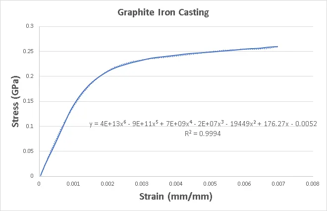
With this new function we ask for 35 points distributed across the graph each 0.02 % strain

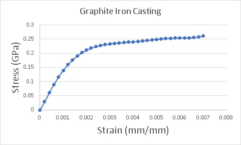
In order to input these data points into Ls-Dyna as a MAT024 material model, we must convert the engineering stress/strain values into true stress and effective plastic strain. To do so, we must use the following equations:

Once everything is prepared, we can proceed to import the dog-bone test specimen to Ls-PrePost

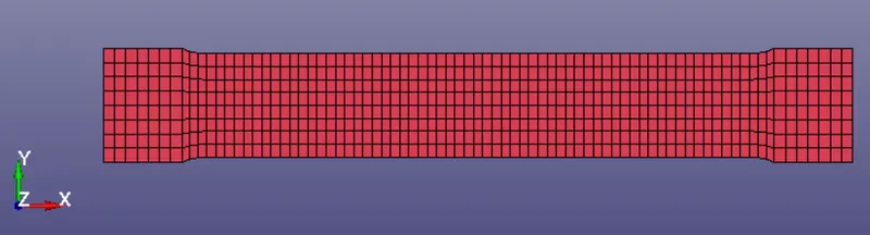
The first step into creating the material card is to define the curve of effective plastic strain vs true strain. In this case, we should only input the values past the yield strength of the material ( 0.14 MPa)

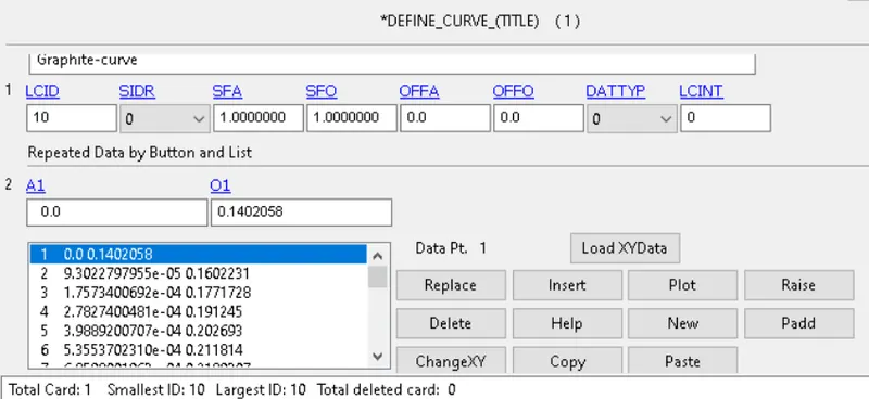
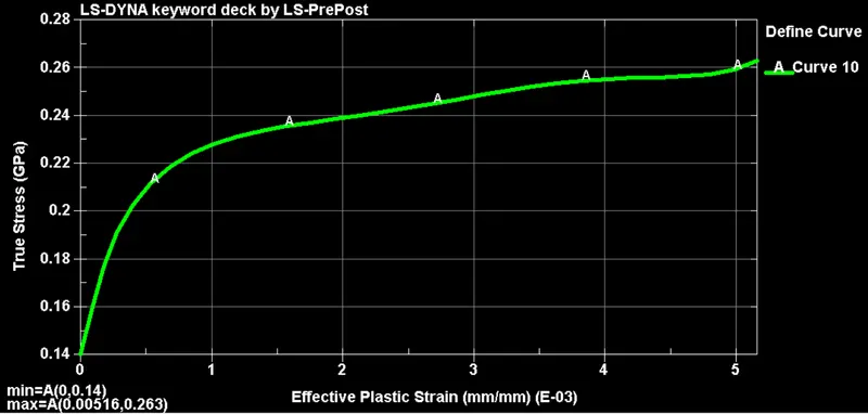
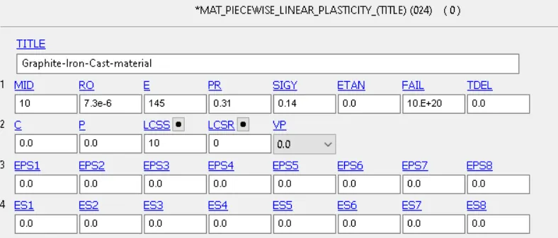
Then, we can proceed to select the MAT024 keyword an input the values obtained from the interpolated data. It's worth mentioning that this material requires both a density and poison's ratio value, which will be taken from generic data on graphite cast iron.

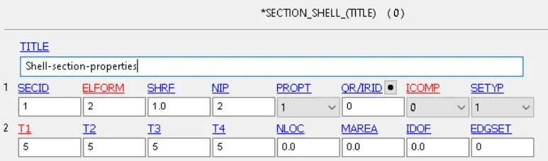
The next step is to define the section properties of the shell elements, and assign both the material and the section properties to the tensile test part

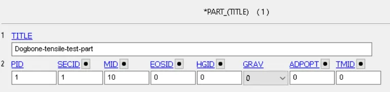
By using the length of the part (145mm), the maximum engineering strain (0.007 mm/mm) and the initial velocity (30mm/min) we can calculate the termination time of the simulation:

From here we can proceed into creating boundary conditions. Which will include:

• A prescribed motion of 1.015mm at a 30mm/min speed (this can be controlled using a define curve keyword)

• Fixed translations in the X and Z axis, as well as fixed rotations in all axes for the edge nodes

• Fixed Y translation for the middle nodes of the tensile test specimen

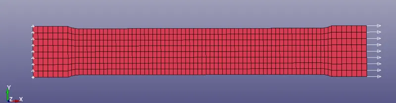
Since the time is very long, this simulation can be considered as a quasi-static case and therefore an implicit simulation scheme is more effective.

To do so, we simply have to add the following set of keywords:

• Control Implicit General ---> Activates Implicit solution scheme
• Control Implicit Auto --> Enables auto time step adjustment during the simulation
• Control Implicit Solution --> Enables the non-linear solver
• Control Implicit Solver --> Enable the liner solver

The last step before running the simulation is to specify our outputs as both D3PLOT and ASCII files

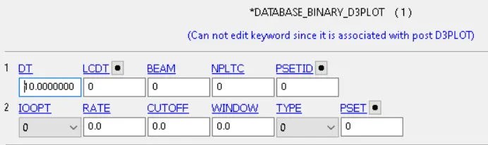
In terms of our ASCII outputs we will only go for:

• GLSTAT ---> Energy summary of the simulation
• MATSUM --> Specific material energy
• SLEOUT --> Sliding energy output
• ELOUT --> Element information output

Simulation Results

The X-stress distribution of the tensile test can be observed both in the following figure/video:

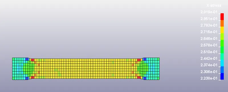
As expected, the largest stresses developed in the regions near to the fillets, which act as stress concentration points. By selecting an element in the center of the tensile test we can obtain both the stress and strain distribution

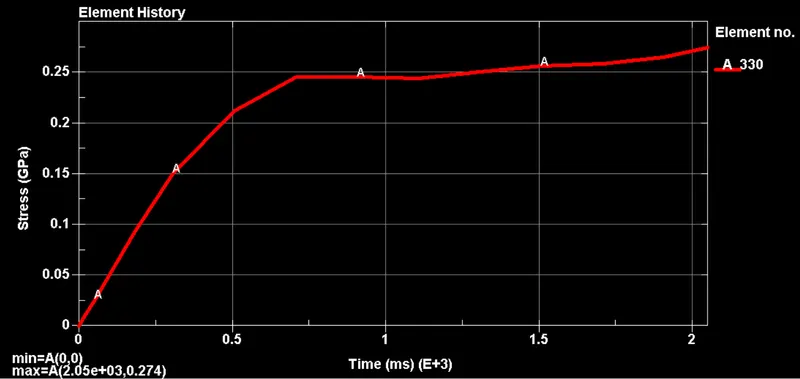
If we export this data and combine it, we get a stress-strain curve which we can compare against the original model

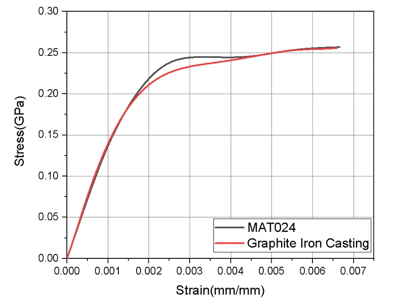
As observed in the previous figure, the region between 0.18% and 0.4% strain presents higher stresses than the original material model. This can be attributed to several things such as:

• Geometry of the test specimen
• Assumed values of poison's ratio and density
• Mesh size

Additionally, other material models such as MAT018 may offer better correlation in that particular zone

Conclusions

• MAT024 (Linear Plasticity model) offers an efficient way to model material behavior past the elastic limit

• The differences between the material model and the raw stress-strain data can be attributed to: Geometry differences between the test specimen and the one used in the simulation; Assumed values of density and poison's ratio; Mesh convergence