Week - 9 Material Modeling from Raw Data

MATERIAL MODELLING FROM RAW DATA

AIM :

• By using the diagram of the true stress-strain curve given for graphite iron casting and creating a material model for the dog bone specimen by using LS-prepost.
• Validating the material model by performing a tensile test on a dogbone specimen.

OBJECTIVE :

• To extract the data from the given stress strain diagram by using data digitizer.
• To clean the data and visually confirm that it matches the original data.
• To convert the data to (kg-mm-ms) unit system
• To process the data and create the material MAT_024 or MAT_018.
• To use the material model (MAT_024 or MAT_018 ) with a dogbone specimen and validate the results.

GIVEN DATA :

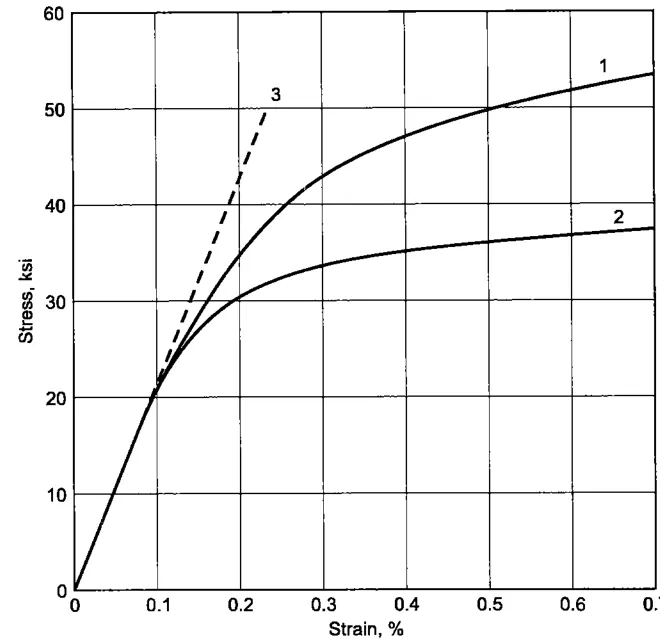
(i) Stress strain diagram of Graphite iron casting material.

(ii) K file of FE model of dogbone specimen.

(iii) Elastic modulus = 20.9E+06 psi.

SOFTWARE USED :

• Data digitizer.
• LS-Prepost 4.7.17 and LS-Run 1.0.100838.

PROCEDURAL STEPS :

STEP 1 :Extraction of datas from the given stress strain diagram.

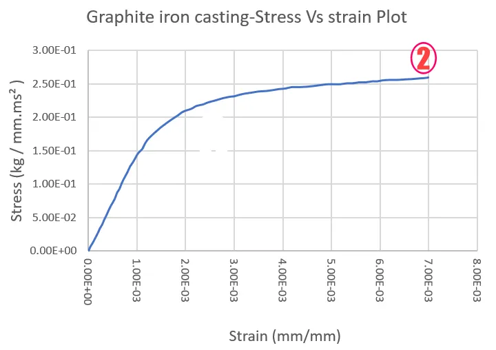
1. I had selected the 2nd curve in the given stress strain diagram and to extract the datas by using data digitizer software.
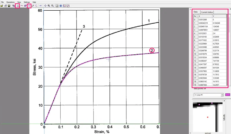
2. First of all to convert the png format of stress strain diagram into jpeg format, because data digitizer supports jpeg formats and other. but not supported png format image file.
3. Then imported the jpeg file of stress strain diagram in data digitizer software.
4. Used scale option in DD, to pick and check the Xmin,Xmax,Ymin & Ymax values.
5. Then click the point capture mode , to selected the every point on the 2nd curve.got the stress and strain values for that corresponding selection.
6. now exported that datas in excel format and saved it.

STEP 2: Convertion of Extracted datas into Kg-mm-ms unit system.

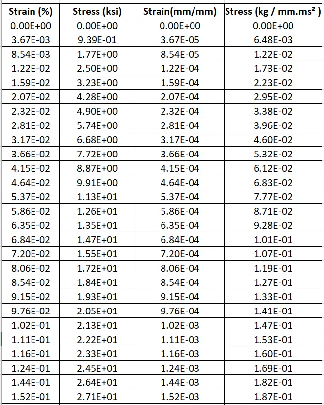
1. Strain values (%)is converted into actual values (mm/mm) by the multiplication of percentage of stain value and 10⁻².
2. Strain (mm/mm ) = strain value (%) X 10⁻² .
3. Stress values (Ksi) is converted into (kg/mm.ms²) by the muliplication of Stress values (Ksi) and 0.0068947573.
4. Stress (kg/mm.ms²) = Stress values (Ksi) X 0.0068947573.

STEP 3: Inspection of extracted stress-strain plot with given stress strain plot.

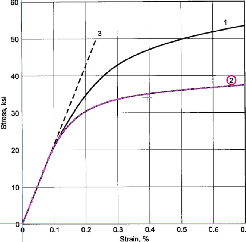
1. Visually confirm that extracted stress-strain plot with given original plot.
2. From the above table in excel plotted the scatter line chart between stress and strain curve is matched the original stress strain plot.

Original Stress Vs strain Plot Extracted Stress Vs strain plot

STEP 4 : To findout effective stress and effective plastic strain.

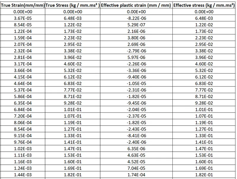
1. The true stress and true strain values are converted into Effective stress and Effective plastic strain value using the following formula.

   Effective stress = True stress

   Effective plastic strain = True strain - (True stress / E)

Given Youngs modulus(E) = 20.9E+06 psi = 144.10 kg/mm.ms².

2. Then calculated the effective stress and effective strain values from the true stress and true strain values from extracted datas.

3. Now in excel sheet plot the graph of effective stress and effective strain values from the above table.

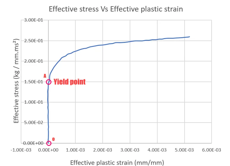
From the graph,

line OA - Stress is directly proportional to strain , so linear line within the proportional limit.

Point A - End of the elastic region , Begining of the plastic region thats an yield point.

from the graph yield point = 0.15 kg/mm.ms²

STEP 5: Import the K file of dogbone specimen.

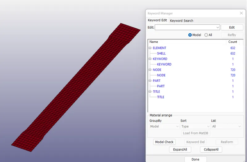
1. Imported the K format type of file using LS-Prepost software.
2. File > Import > LS-Dyna keyword file > browsed to selected the K type of file > imported it.
3. In order to check the keywords contained in the file we have to follow the below steps.
4. Side bar > model and part > keyword manager > checked the model.

STEP 6: Creation of material card.

1. To assign the material card for dogbone specimen by the following steps.
2. I had prefereed to choose material type is MAT_024 (MAT_PIECEWISE_LINEAR_PLASTICITY)
3. This is Material Type 24, which is an elasto-plastic material with an arbitrary stress as a function of strain curve and arbitrary strain rate dependency can be defined.
4. Side bar > model and part > keyword manager > MAT > all > MAT_024.
5. Created new ID is 1 and give title is dogbone_graphite_iron_casting material and specified the properties values as Kg-mm-ms unit system.

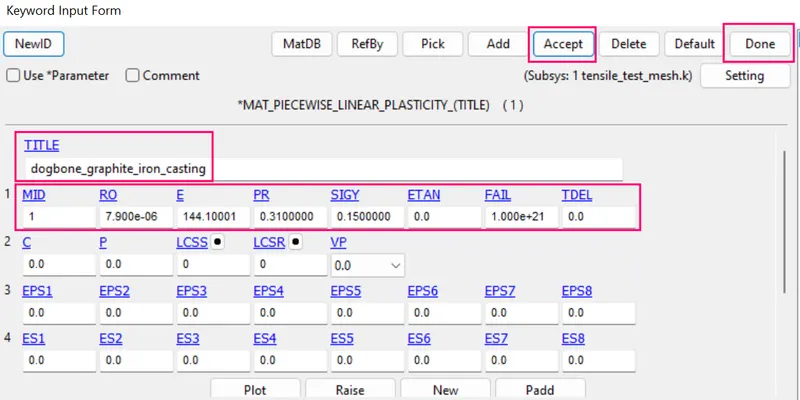
Where,

1. Ro - density of the garphite iron casting = 7.9*e-6 Kg /mm³.
2. E - youngs modulus = 144.10 kg/mm.ms².
3. PR -poissons ratio= 0.31
4. From the graph Yield stress(SIGY) = 0.15kg/mm.ms²

STEP 7: Creation of section card.

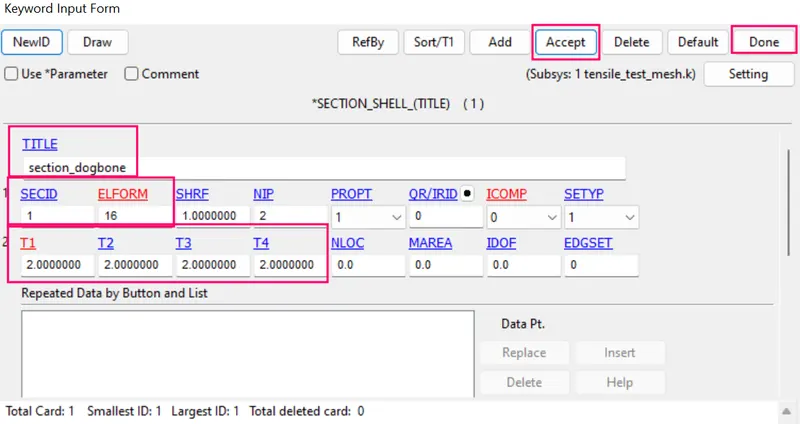
1. In this section element formulation ,integration rule ,nodal thickness and cross sectional properties are defined.
2. Created the section shell for dogbone specimen.
3. Side bar > model and part > keyword manager >all > section >specified the thickness value is 2 mm > accept and done.

STEP 8: Assign material card and section card to the dogbone specimen part.

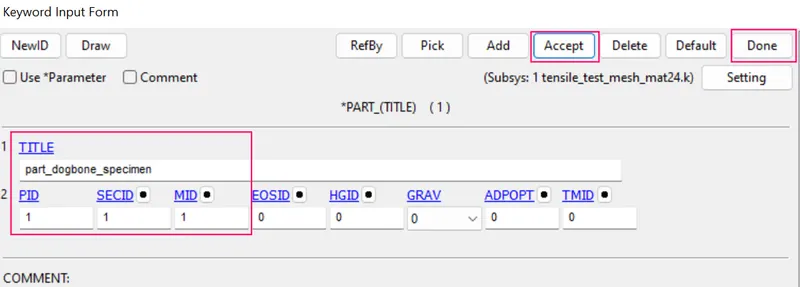
1. Inorder to create the dogbone specimen part by the following steps.
2. Side bar > model and part > keyword manager >model > part > assigned the MID and SECID cards to dogbone specimen part >accept and done.
   

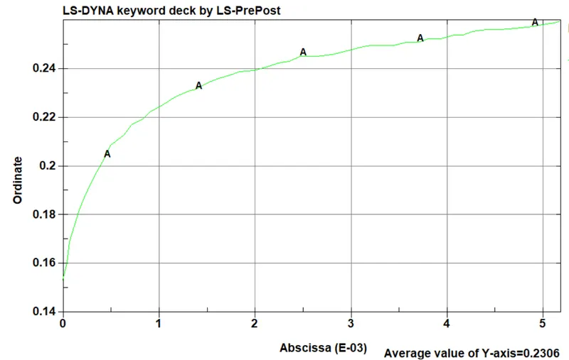
STEP 9: Define a curve.

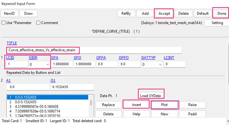
1. Define a curve [for example, load (ordinate value) as a function of time (abscissa value)], often loosely referred to as a load curve. The ordinate may represent something other than a load however, as in the case of curves for constitutive models.
2. Before define a curve , we have to copy the effective stress and effective strain values (consider only beyond yield point data) in excel sheet and saved as CV(coma delimited) format.and also deleted the neagtive values of effective plastic strain coressponding effective stress values.
3. In order to define a curve by the following steps.
4. Side bar > model and part > keyword manager >define > curve > LCID is 1 > import the CV format XY data > insert > accept and done.

STEP 9: Define a boundary condition.

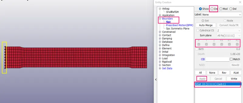
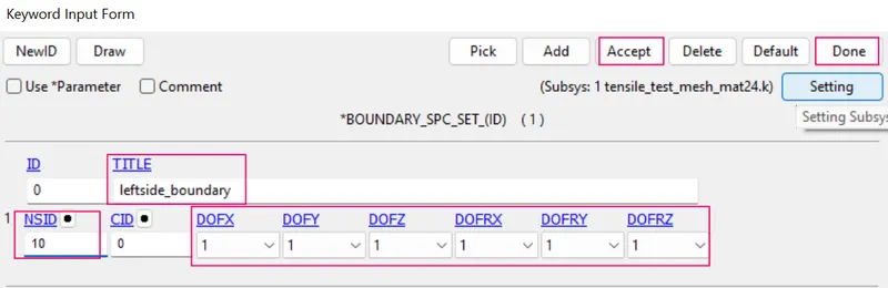
STEP 9A: Define a boundary condition at fixed end nodes of the specimen.

1. The nodes at the fixed end is constrained in the Y and Z direction only and the X direction is not constrained because of expansion during the tensile test.
2. Inorder to create boundary condition by the following steps .
3. Sidebar> model > create entity > boundary > spc > create > selected the node by path > nodes at the fixed end is constrained in the Y and Z direction only and the X direction is not constrained > apply and one.

STEP 9B : Define a precribed motion boundary condition at free end nodes of the specimen.

STEP 9B(1) : Define a curve for precribed motion.

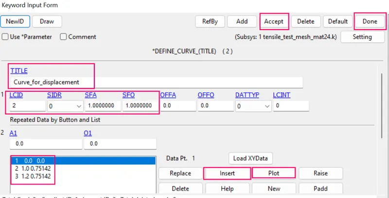
1. Before creation of prescribed motion at free nodes of the specimen we need to define a load curve for that prescribed motion.
2. In order to create a curve by the following steps.
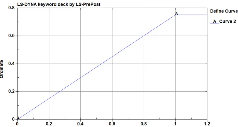
3. Displacement =Effective plastic strain X length of the dogbone specimen( 5.18E-3 x 145= 0.75mm)
4. Side bar > model and part > keyword manager >define > curve > LCID is 2 > specify XY data > insert > accept and done.

STEP 9C(2) : Creation of node set for the displacement at free end of the specimen.

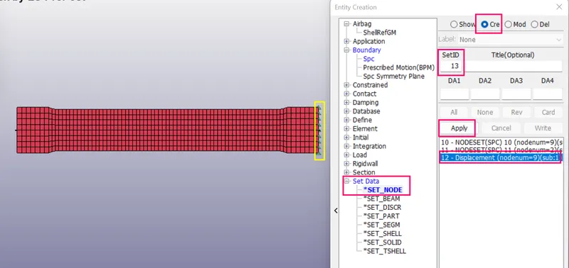
1. In order to create the node set by the following steps.
2. Sidebar > model > create entity > set data > set node > selected the nodes at free end of dogbone specimen > apply and done.

STEP 9C(3) : Assign the Nodeset id and load curve to the boundary precribed motion set.

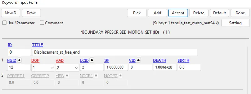
1. In order to create the prescribed motion set at free end by the following steps.
2. Side bar > model and part > keyword manager > BOUNDARY_PRESCRIBED_MOTION_SET > assigned nodeset id 12 , DOF is 1 , VAD is 2 and assigned load curve for displacement LCIDis 2 > accept and done.

IMPLICIT ANALYSIS
Now run this file using an implicit solver. Additional control implicit cards are used to run this simulation in an implicit solver.

STEP 10: Define a control cards
Simulation of implicit analysis and define related control parameters such as CONTROL_IMPLICIT_GENERAL , CONTROL_IMPLICIT_SOLUTION ,CONTROL_IMPLICIT_SOLVER & CONTROL_IMPLICIT_AUTO.

STEP 10A : Define a CONTROL_IMPLICIT_GENERAL card.

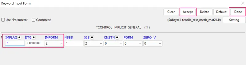
1. In order to create control implicit general card by the following methods.
2. Sidebar > model > keyword manager > all > CONTROL > IMPLICIT_GENERAL >IMFLAG is 1 (implicit analysis) and dt) IS 0.05 and other parameter remain same > accept and done.

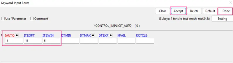
STEP 10B : Define a CONTROL_IMPLICIT_AUTO card.

1. In order to create control implicit auto card by the following methods.
2. Sidebar > model > keyword manager > all > CONTROL > IMPLICIT_AUTO > parameters remain same as per default values > accept and done.

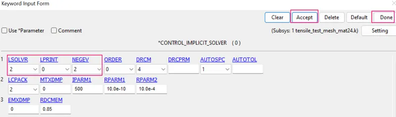
STEP 10C : Define a CONTROL_IMPLICIT_SOLVR card.

1. In order to create control implicit solver card by the following methods.
2. Sidebar > model > keyword manager > all > CONTROL > IMPLICIT_SOLVER > LSOLVR is 2( Parallel multi-frontal sparse solver ) and other parameters remain same as per default values > accept and done.

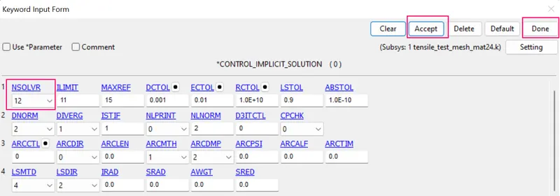
STEP 10D : Define a CONTROL_IMPLICIT_SOLUTION card.

1. In order to create control implicit solutionl card by the following methods.
2. Sidebar > model > keyword manager > all > CONTROL > IMPLICIT_SOLUTION >NSOLVR is 12 (nonlinear ) and other parameters remain same as per default values > accept & done.

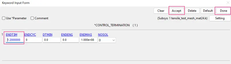
STEP 10E : Define a CONTROL_TERMINATION card.

1. The main purpose of control termination card is to stop the job.
2. In order to assign the control termination card by the following steps. 3. Side bar > model and part > keyword manager > control > termination > specify termination time is 1.2 ms > accept and done.

STEP11: Define the outputdatabases.

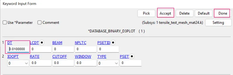
STEP11A :To define the output database as Binary D3 plot.
1. DATABASE_BINARY_D3PLOT ensures d3 plot files which its stores stress strain contour of the entire deformed model.
2. In order to create the DATABASE_BINARY_D3PLOT by the fllowing steps.
3. Side bar > model and part > keyword manager > database > select DATABASE_BINARY_D3PLOT > DT value is 0.01 ms is a time interval between output states > accept & done.

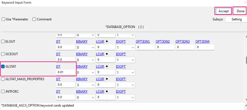
STEP11B :To define the output database as ASCII.

1. ASCII can generate different outputs such as force generated in a contact like total energy and material energy etc.
2. In order to create the ASCII by the fllowing steps.
3. Side bar > model and part > keyword manager > database > select ASCII_option > check GLSTAT ,NODOUT >specify all DT value is 0.01 > accept & done.

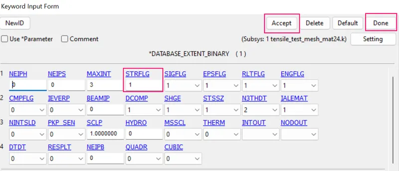
STEP 11C :To define the output database as extend Binary.
1. Now we have everything for the simulation but to extract the results we need to create a database cards for the model.
2. We also need to generate the strain outputs. To do that, we can create a keyword by going to Keyword manager and selecting DATABASE > EXTENT_BINARY.
3. To create the database extend binary card by the following steps,
Side bar > model > keyword manager > all > DATABASE > EXTEND_BINARY> and give STRFLG as ‘1’, this is due to extract the true strain values for the model and accept the card .

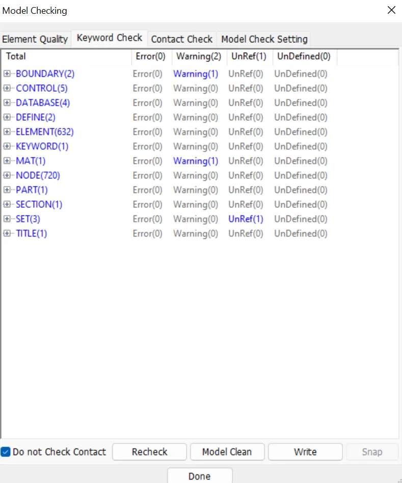
STEP12: Model checkup
1. The model is checked for any errors before solving using model checker.
2. After all the errors are cleared, the drop test setup is saved and is ready to run in LS DYNA manager for solving the scenario.
3. Warnings we can ignore ,once model check is run , it will look like as shown in picture below.

STEP 13 : Run the simulation.
1.. To run the using LS-run by the following steps.
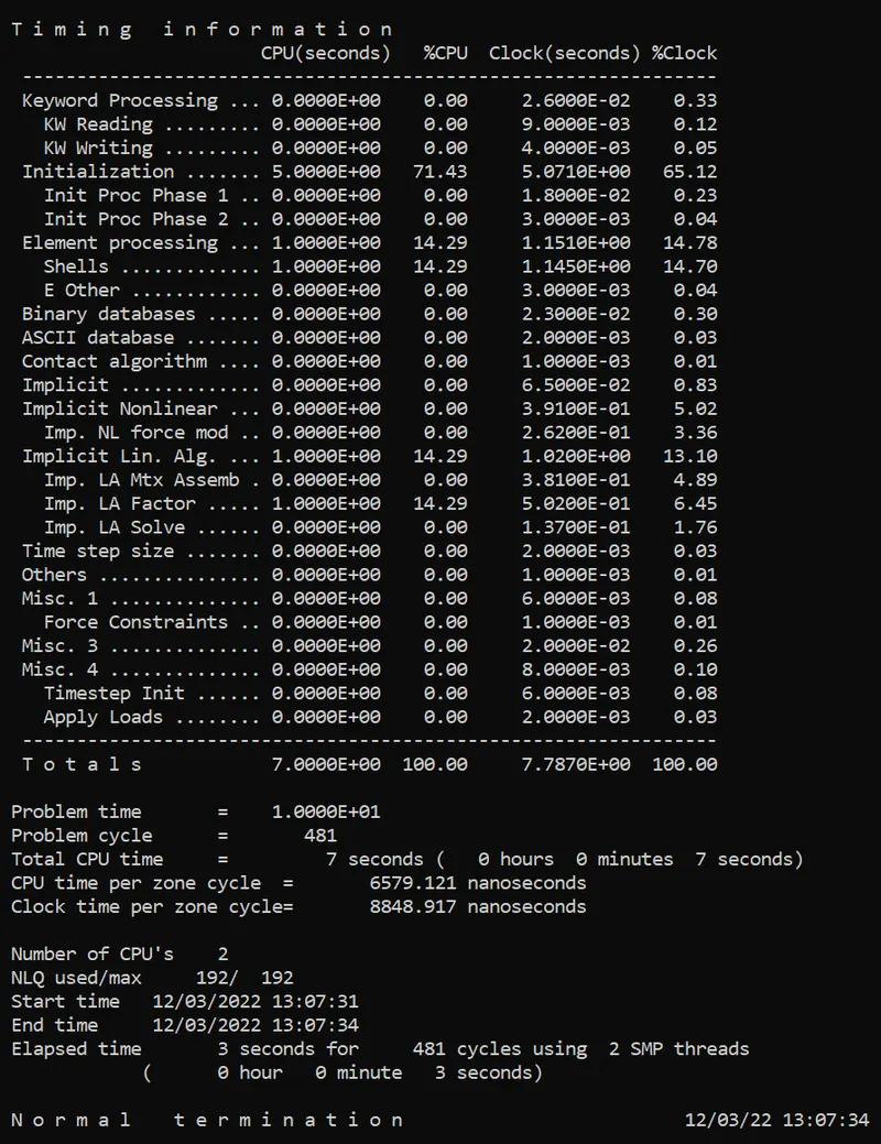
2. Title bar > file > run LS-dyna > runned the k file of tensile_test_mesh_mat24 > achieved normal temination. it means the model is ready for post processing.
3. During simulation run window will popup as shown in picture below,

STEP 14 : POST PROCESSING
1. In order to see simulation results , we have to open output file in LS-Prepost by the following steps.
2. In LS-prepost -Title bar > file > open > LS -Dyna binary plot > selected the d3 plot file > visibled to see animation file.
3. For plot the stress contour , go to sidebar > post >fringe component > selected in which results need for analysing the problem.

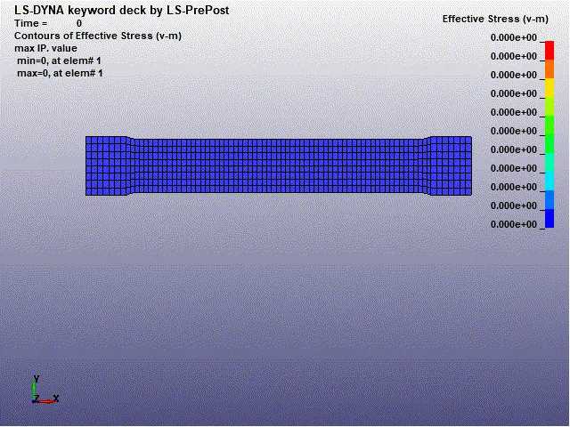
(a) Contour plot of vonmisses stress of tensile test of dogbone specimen.

Max effective stress = 0.2571 kg/mm.ms²

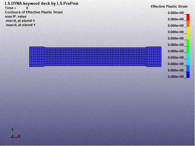
(b) Contour plot of effective plastic strain of tensile test of dogbone specimen.

Max effective plastic strain = 0.0053 mm/mm

(c) Effective stress Vs Effective plastic strain plot of tensile test of dogbone specimen.

Time Vs Effective stress

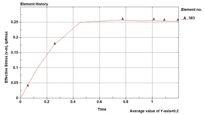
• The highest stress value 0.254 kg/mm.ms² is observed in element no 383 as shown in the above plot.

Time Vs Effective plastic strain

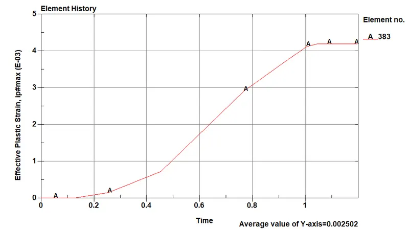
• The highest plastic strain value 0.00419 mm/mm is observed in element no 383 as shown in the above plot.

Effective stress Vs Effective strain

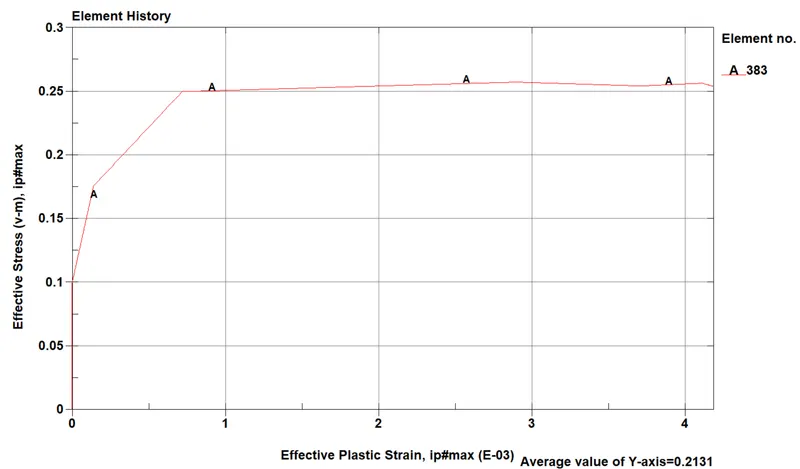
(d) Comparison of raw effective stress Vs strain and Simulated effective stress Vs strain.

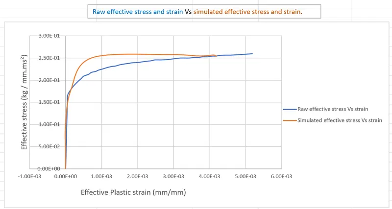
From the Comparison of above plots,

Raw datas

Max effective stress reached = 0.26 kg/mm.ms²

Max effective strain reached = 0.00518 mm/mm.

Simulated datas

Max effective stress reached = 0.254 kg/mm.ms²

Max effective strain reached = 0.00419 mm/mm.

From above data we can observe that the graph values, raw values of 2nd curve and simulated values are almost equal to we can say that our material model is correct.

CONCLUSION

• This simulation objective has been achieved as a close to accurate material card (MAT_24 piecewise linear elasticity) has been verified for the graphite iron tensile test through verification of both physical and simulation results.