Week - 9 Material Modeling from Raw Data

1. Extract the data from the diagram 
2. Clean the data and visually confirm that it matches the original data and the elastic modulus is 20.9E+06 psi.
3. Convert the data to (kg-mm-ms) unit system
4. Process the data and create the material as demonstrated
5. Use the material model with a dogbone specimen and validate the same.

Aim-

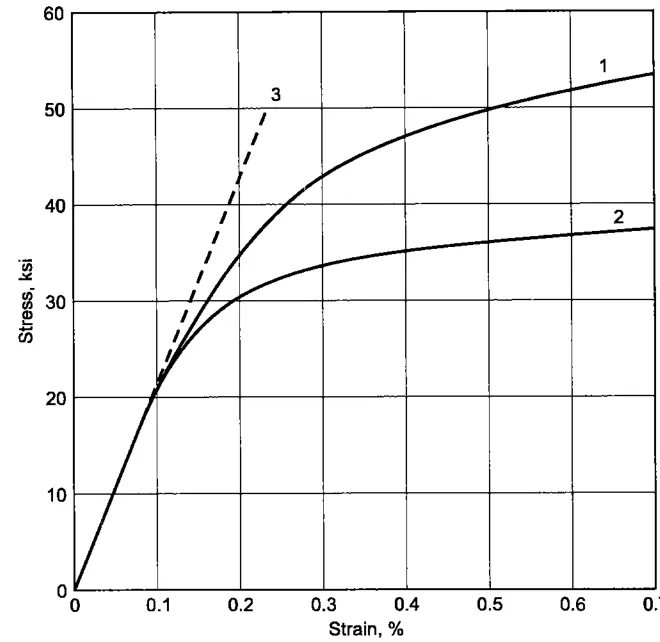
• This challenge aims to extract two different material properties for the same material with varying alloys from below the curve. Then we have to verify the materials with output curves.
  •  

Procedure-

1. The first step is to open the above image in the data digitizer UI, then we have to trace both curves and extract the values in excel format. The data extracted from the digitizer is % strain and stress in ksi which need to convert to strain and stresses to GPa. Then the engineering stress is converted to true stress.
   •  
2. The next step is to convert the engineering stresses to true stress
   • true strain `epsiunderset(true)()=ln(1+sigmaunderset(true)())`
   • true stress `sigmaunderset(true)()=sigmaunderset(eng)()*exp^(epsiunderset(true)())`
3. Then the next step is to convert true strain into effective plastic strain by using below formula
   • Effective plastic strain`epsiunderset(eps)()=epsiunderset(true)() -(sigmaunderset(true)())/E`
   • `sigma`= stress
   • `epsi`= strain
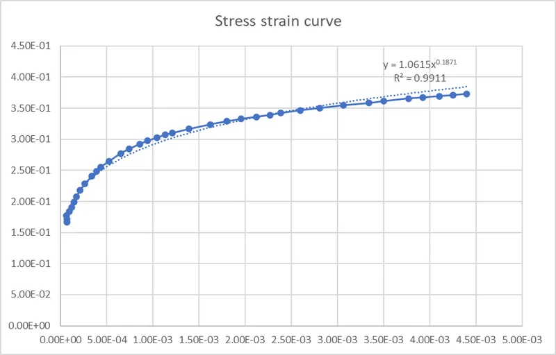
4.  After that we have to plot the curve between effective plastic strain and true stress, then check for good cuve fit with R square % more than 99%.
   • 
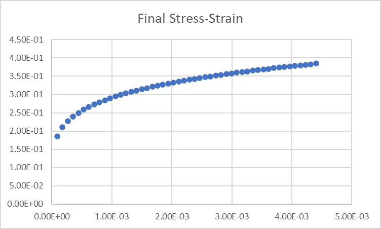
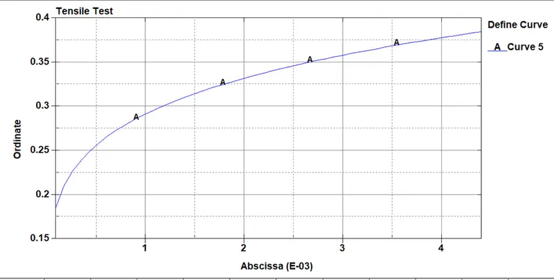
5.  Next we consider fifty values between the maximum and minimum strain value and calculate the stresses using the curvefit function. Now the plot becomes
   • 
6. Now we save the final values in a csv file to use it as material data in material card.
7. The next step is to open the dog bone model in ls-prepost.
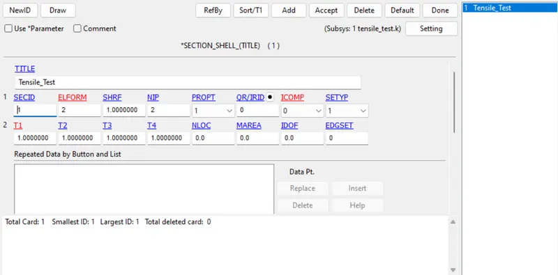
8. First we have to define the section card which is shell card with elform 2 with thickness as 1.
   •  
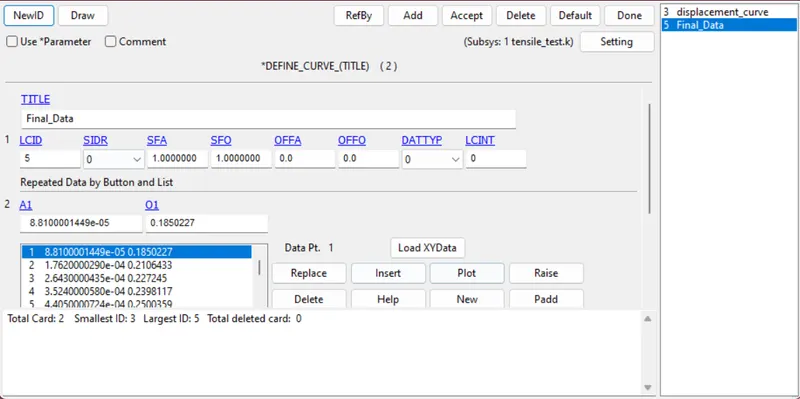
9. The next step is to define the curve Id for material card which has to be given as input.
   • 
   •  
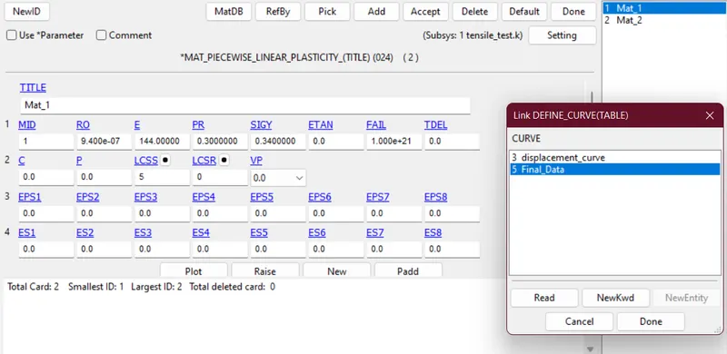
10. The next step is to define the material card where we have to give input the curve id as the material property. Also we have to give input the density and young's modulus which has been calculated while cleaning the digitizer data which is 144 GPa.
    •  
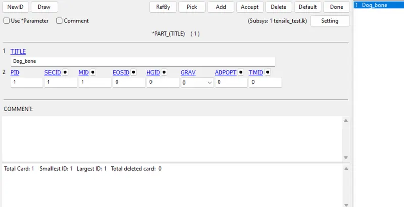
11. Next step is to give reference the mate card and section card in part card.
    •  
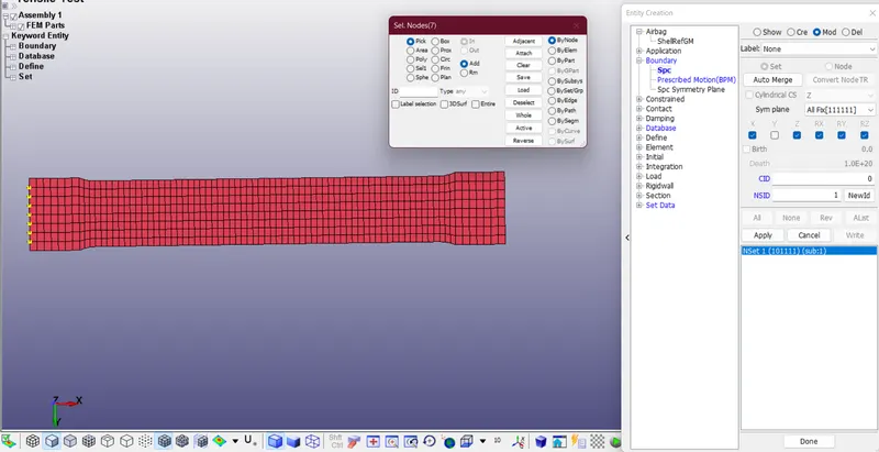
12. The next step is to give the boundary condition to the dog bone to perform the appropriate tensile test. For this it is necessery to fix one end of dogbone and give some kind of load at other end it can be imposed velocity or displacement.
    • Fixed end card is given below
      • 
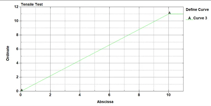
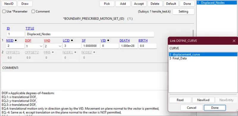
    • For load here prescribed motion set has been applied at the other end of the dog bone and load is given as displacement in time step on x direction.
      • Displacement curve is given below
        • 
      • The prescribed motion card is given below
        • 
13. The next step is to define the database first is 
    • The ASCII options in which the selected options are MATSUM, GLSTAT, NCFORCE, NODEOUT.
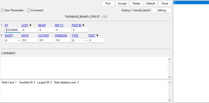
    • Then Binary plot is selected and the card is given below
      • 
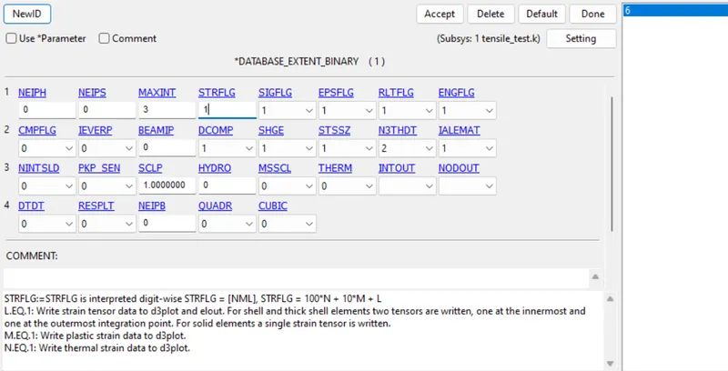
    • To get integer point strain value the Extent Binary option has been enabled and STRFLG is changed to 1. The following card is given below
      • 
14. The next step is to define Control cards such as Hourglass, Termination and Timestep 
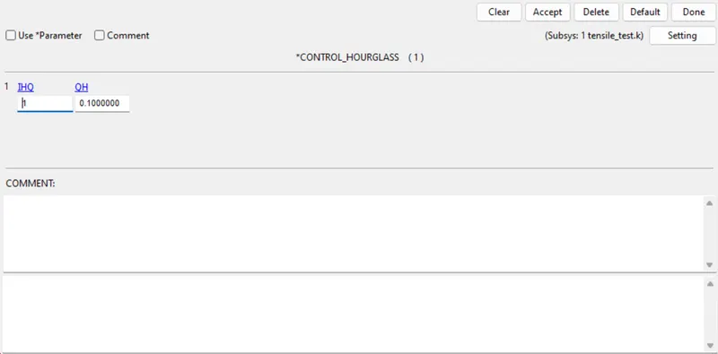
    • Hourglass card is to control the hourglass effect caused in reduced integration scheme of element selection. The card is given below
      •  
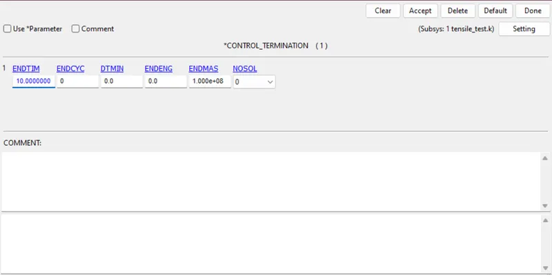
    • In termination card the time periond of analysis is defined and the card is given below
      • 
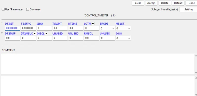
    •  In timestep card the interval of analysis is given below which is 0.01 in our case
      • 
15.  When the simulation runs we can open the d3plot can see different plots.
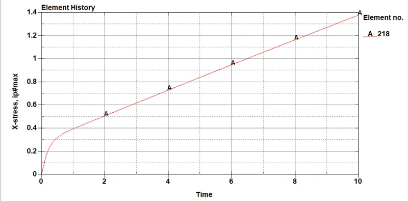
    1. First consider the stress vs time plot for an element in the middle section of the dog bone
       • 
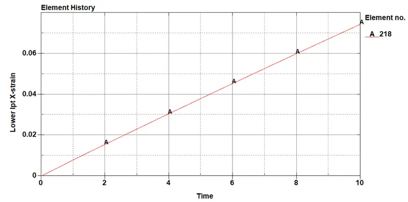
    2. The plot between lower ipt strain vs time is given below
       • 
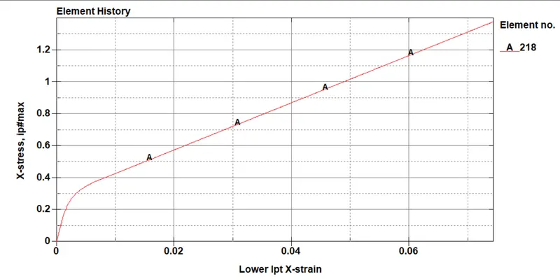
    3. Now we can cross plot between X-strain and X-stress, the plot is given below
       • 
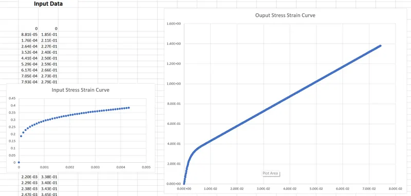
16.  Now let's check this plot with the input plot 
    • Both the curve has different domain but behave in similar manner
      • 

 Conclusion

• The output modeled data behaves in a similar way as the input model data.
• I've learned cleaning raw data and creating cleaned stress-strain data.
• All the files are attached below.