Week - 9 Material Modeling from Raw Data

Aim:

The aim of this challenge is to learn the material modeling procedure in any FEA software by carrying out the validation of the material data input against the data obtained from FEA simulation. Here the input material data is given in the form of an image of the stress-strain curve, from which the data needs to be extracted and fed into the solver. Finally the stress-strain graph obtained from the simulation needs to be compared with the given graph to validate the same.

Explanation:

First the Get data digitizer was downloaded and installed.

Then the given image was converted into the .jpeg format to open it in Get data digitizer.

In Get Data Digitizer, the scale was selected using the “Set the Scale” option, in which maximum and minimum values along the X and Y axes were selected and input.

The curve 1 was decided to be used for the analysis.

Then the “Point capture mode” was used to select points on the curve 1 to map it accurately. The data was then exported to a text file. From the text file the data was copied to Excel.

In Excel, under the Data tab, Text to column option was used to separate the data into 2 separate columns. But the stress values were in psi, which needed to be converted to the kg-mm-ms unit system.

The formula for unit conversion was entered into excel and the stress units were changed, first from psi to Pa and then from Pa to kg/mm.ms2.

1 Pound (force) = 1 pounds * gravitational acceleration

= 1 pounds * 32.174 ft/s2

= 0.4536 kg * 32.174 * 0.3048 m/s2

= 4.448 kg.m/s2

= 4.448 N

1 psi = 1 pound-force/sq.inch

= 4.448 N/ (0.0254)2 m2

= 4.448 / 0.00064 N/m2

= 6950 kg/m.s2

= 6.95 e-6 kg/mm.ms2

The values thus obtained are the true stress and true strain values.

The material card used is MAT_024 “Piecewise Linear Plasticity”. In this card the stress strain values are provided by a load curve. Hence under the LCSS tab, the load curve ID 1000 was chosen. Here the data needs to be as effective stress (true stress) and effective plastic strain.

Hence the strain values from the given graph were converted to effective plastic strain, using the following equation:

Effective plastic strain = total true strain - (true stress/Young’s modulus)

Then the given .k file was opened in LS-PrePost.

Then the *DEFINE_CURVE was used to create a curve describing the stress-strain relationship. But, here, only a1=0 and o1=0 were input. And the .k file was saved.

Later the .k file was opened in Notepad++ and the data obtained from the given graph was inserted under the *DEFINE_CURVE keyword. The .k file was saved.

Then again the .k file was opened in LS_PrePost and the rest of the model was built by providing Part, Section and Material definitions as well as the boundary conditions and control parameters.

The part was given the SHELL section with Elform 2. It was assigned the material defined in the MAT-024 card above.

For boundary conditions, the set of nodes at one end of the specimen were fixed in 5 DOFs and the translation DOF in Y-axis was allowed to model lateral compression during the tensile test.

The nodes at the opposite end of the specimen were provided a displacement in positive X-direction using *PRESCRIBED_MOTION_SET keyword.

The curve for displacement was also defined using *DEFINE_CURVE. For this the value of displacement was obtained from the highest strain value in the given graph. The highest true strain value was converted to engineering strain. The engineering strain was then multiplied with the length of the specimen to obtain the change in length of the specimen. This value of change in length was used as the displacement value in the *DEFINE_CURVE. Thus, the displacement of 1 mm was given with the end time of 10 ms.

The formulae used for conversion were:

Engineering strain = e^(true strain) - 1

Change in length = Engineering strain * Original length of the specimen

In the control parameters, *HOURGLASS keyword was used to avoid hourglassing of SHELL elements.

*CONTROL_IMPLICIT_GENERAL was used and IMFLAG was set to 1 to use the Implicit method of analysis. The DT0 was set as 1 ms.

*CONTROL_IMPLICIT_SOLUTION with default parameters was also used.

The End time of the run was set to 10 ms using *CONTROL_TERMINATION keyword.

*DATABASE_BINARY_d3plot was used to get d3plot as output with DT of 1ms.

*DATABASE_HISTORY_NODE was used to get output data at a particular node and in ASCII options NODOUT with DT of 1 ms was used.

The simulation was run. It ran smoothly and there was normal termination.

Then the d3plot file was opened in LS-PrePost. From the Right hand side toolbar the History option was selected, in which the Element option was selected. An element from the middle of the specimen was chosen and the time-history graphs for stress and strain were plotted.

In the graph’s window, the Save option was selected, in which the Interpolate option was ticked and 20 interpolation points were requested. Then the file was saved. The files were saved as text files.

The data from the text files of stress and strain plots was then copied into Excel and the stress vs. strain graph was plotted.

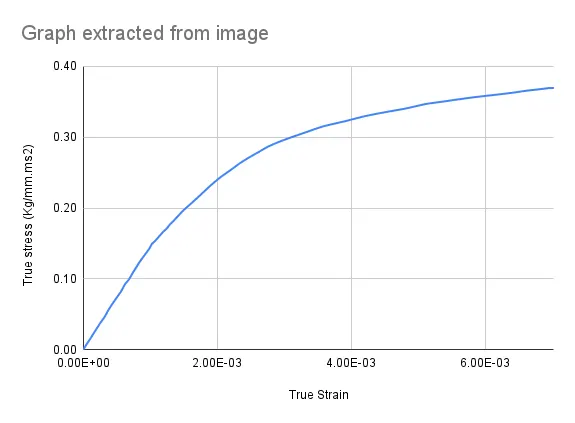
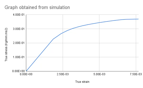
The graph obtained from the given image and the graph obtained from the simulation are provided below for the comparison.

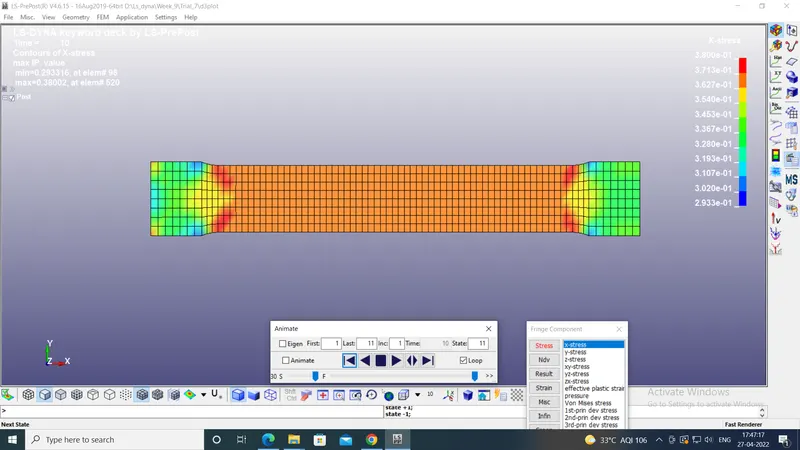
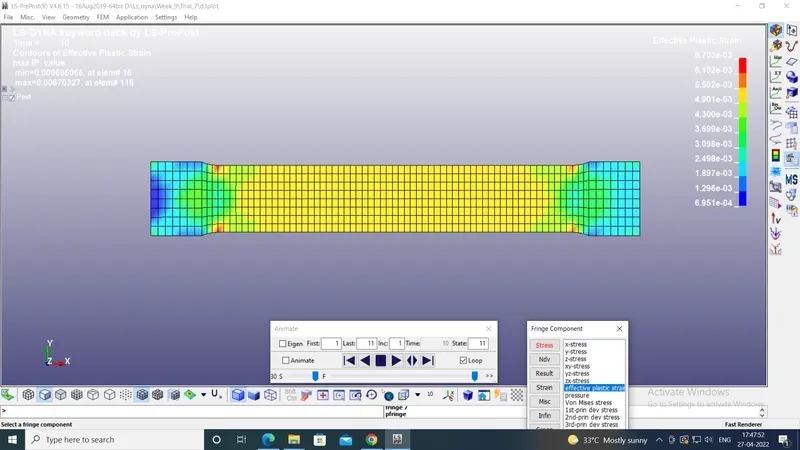
The stress and strain distribution plots are also provided below:

Conclusion:

It can be seen, that the stress-strain graphs of the input and output data are matching almost perfectly. This validates that the material card used is apprpriate for the given simulation. The challenge also provided a lesson on how to use material curves to define the material behaviour. The results also imply that the model was also constructed accurately, in terms of boundary conditions, control parameters and part & section definitions. Thus the challenge also provides an example of the method, which can be used to establish the accuracy of the model during post-processing.