Week - 2 - Explicit and Implicit Analysis
Aim: The aim of this report is explain, in detail, the difference between the explicit and implicit methods of the finite element analysis (FEA). The report contains calculations and corresponding graphs to compare the two methods.
Explanation:
1. Explicit method: This method uses the values obtained in the previous iteration to approximate the results for the next iteration. This can be explained by following calculations:
Here given Force F(u)=`u^3+9u^2+4u` Stiffness coefficient k= 3u^2+18u+4
Taking external force dF(e) = 1N
Iteration 1 :
Initial displacement u(0) = 0 Stiffness coefficient k(0) = 4
Incremental displacement du(1) = dF(e)/k(0) = 1/4 = 0.25 u(1)=u(0) + du(1)=0.25
F(u1)=1.5781
Iteration 2:
k(1) = 3u(1)^2+18u(1)+4=0.1875+4.5+4= 8.6875 k(1)=8.6875
du(2) = dF(e)/k(1) = 1/8.6875 = 0.1151 u(2)=u(1)+du(2)=0.25+0.1151 u(2)=0.3651
F(u2)=2.7086
Iteration 3:
k(2)=3u(2)^2+18u(2)+4=0.3993+6.5718+4 k(2)=10.9711
du(3)= dF(e)/k(2)=1/10.971=0.0911 u(3)=u(2)+du(3) u(3)=0.4562
Now internal force F(u)=u(3)^3+9u(3)^2+4u(3) = 3*0.0949+9*0.2081+4*0.4562 =0.2847+1.8729+1.8248=3.9824
F(u3)=3.9824
| Iteration | dF(e) | du | u | F(e) | F(u) | R=F(u)-F(e) |
| 1 | 1 | 0.25 | 0.25 | 1 | 1.5781 | 0.5781 |
| 2 | 1 | 0.1151 | 0.3651 | 2 | 2.7086 | 0.7086 |
| 3 | 1 | 0.0911 | 0.4562 | 3 | 3.9824 | 0.9824 |
As can be seen, the method uses the values of stiffness coefficient of the previous iteration to calculate the displacement in the next iteration. This causes the final solution to deviate from the actual values. Thus this method gives only approximate results.
To increase the accuracy of this method, the time step needs to be small, as suggested by the Courant-Friedrichs-Levy criterion. This requires more number of iterations.
However, the method needs lesser computing resource, being an approximate method.
2. Implicit method:
In this method, the values from the previsous iteration are not used, instead some elaborate calculations are used to calculate the values, separately for each iteration/time step. This method requires the inversion of the matrix and an identity matrix to find these values. This increases the complexity of the calculations and hence requires greater computing resources.
The method tries to achieve equilibrium in each time step by using a correction factor, foun by using the Newton-Raphson iterations. These iterations calculate the difference called 'resiual' (R) between the actual and calculated values of the variables. The values of R needs to be below the specified tolerance limit, to achieve equilibrium solution.
This is explained using the following example:
Iteration 1:
Here u(0)=0 k(0)=4 dF(e)=1 du(1)=0.25 u(1)=0.25 R(1)=0.5781 k(u1)=8.6875
R>0.001 Hence Newton-Raphson iterations are needed.
Corrected value of du(1) = du(1)' = - R(1)/k(u1) = -0.5781/8.6875=-0.0665
Corrected value of u(1)=u(1)' = u(1)+du(1)' = 0.25-0.0665 = 0.1835
Corrected value of F(u1)= F(u1)' = 0.0061+0.3030+0.734 = 1.0431 R'=0.0431>0.001
k(u1') = 7.404
Corrected value of du(1)'=du(1)" = du(1)' - R'/k(u1')= -0.0665-0.0431/7.404=-0.0723
Corrected value of u(1)'=u(1)"=u(1)+du(1)" = 0.25-0.0723 = 0.1777
Corrected value of F(u1)'= F(u1)" = 0.0056+0.2841+0.7108 = 1.0005 R"=0.0005<0.001
Hence correct value of u(1)=u(1)"=0.1777 and F(u1)=1.0005.
Iteration 2:
Here u(1)=0.1777 k(u1)= 7.2933 dF(e)=1 du(2)=1/7.2933=0.1371
u(2)=0.1777+0.1371=0.3148 F(u2)= 0.0311+0.8918+1.2592=2.1821 R(2)=2.1821-2=0.1821
k(u2) = 9.9636
R>0.001 Hence Newton-Raphson iterations are needed.
Corrected value of du(2) = du(2)' = - R(2)/k(u2) = -0.1821/9.9636=-0.0182
Corrected value of u(2)=u(2)' = u(2)+du(2)' = 0.3148-0.0182 = 0.2966
Corrected value of F(u2)= F(u2)' = 0.0260+0.7917+1.1864 = 2.0041 R'=0.0041>0.001
k(u2') = 9.6027
Corrected value of du(2)'=du(2)" = du(2)' - R'/k(u2')= -0.0182-0.0041/9.6027=-0.0186
Corrected value of u(2)'=u(2)"=u(2)+du(2)" = 0.3148-0.0186 = 0.2962
Corrected value of F(u2)'= F(u2)" = 2.0003 R"=0.0003<0.001
Hence correct value of u(2)=u(2)"=0.2962 and F(u2)=2.0003.
Iteration 3:
Here u(2)=0.2962 k(u2)=9.5948 dF(e)=1 du(3)=1/9.5948=0.1042
u(3)=0.2962+0.1042=0.4004 F(u3)=3.1085 R(3)=0.1085 k(u3)=11.6881
R>0.001 Hence Newton-Raphson iterations are needed.
Corrected value of du(3) = du(3)' = - R(3)/k(u3) = -0.1085/11.6881=-0.0092
Corrected value of u(3)=u(3)' = u(3)+du(3)' = 0.4004-0.0092 = 0.3912
Corrected value of F(u3)= F(u3)' = 3.0019 R'=0.0019>0.001
k(u3') = 11.5007
Corrected value of du(3)'=du(3)" = du(3)' - R'/k(u3')= -0.0092-0.0019/11.5007=-0.0093
Corrected value of u(3)'=u(3)"=u(3)+du(3)" = 0.4004-0.0093 = 0.3911
Corrected value of F(u3)'= F(u3)" = 3.0008 R"=0.0008<0.001
Hence correct value of u(3)=u(3)"=0.3911 and F(u3)=3.0008
| Iteration | dF(e) | u | F(e) | F(u) | R |
| 1 | 1 | 0.1777 | 1 | 1.0005 | 0.0005 |
| 2 | 1 | 0.2962 | 2 | 2.0003 | 0.0003 |
| 3 | 1 | 0.3911 | 3 | 3.0008 | 0.0008 |
Thus it can be seen, that the implicit method provides better results than the explicit method. But it also requires greater computational resources and computing time. Hence it would not be prudent to use implicit method for very complex geometries or analyses.
The two methods have been compared with the exact values in the following plot:
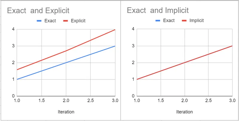
Conclusion
It is clear, that both the methods have their own advantages and disadvantages. Hence a careful choice needs to be mae among the two. The explicit method should be used in very complex analyses like transient dynamic analyses like crash test of a vehicle. It should use smaller time step to obtain better results. On the other hand, the implicit method can be used for simpler analyses like static structural and simpler geometries.