Week - 9 Material Modeling from Raw Data

Aim: To Model a material card from the raw data available, and verify it by comparing the results with input defined.

Objective: To extract the stress-strain data points from the image and input them into ls dyna, and compare the result of the simulation with that obtained from the raw data.

Theory: While modelling a material we focus upon non-linear curve (linear portion is shown by E value) Non-linear curve is easily shown by ls-dyna or while we modelling the material.

To Model a Linear behavior of material, only three independent parameter required E (Youngs Modulus), u (Poisons ratio) and ρ (density for units).

The linear relation as per the straight line is described only by the slope. i.e. E (Youngs Modulus)

When the material enters into the non-linear zone the curve needs to define using the non-linear function according to the way material behaves under different types of loading.

Depending upon the way material behaves, it can be described using constitutive law, such as

Elasto-Plastic material

Hyperelastic material

Viscoelastic material

Actual Process of Modelling a Material card from test data

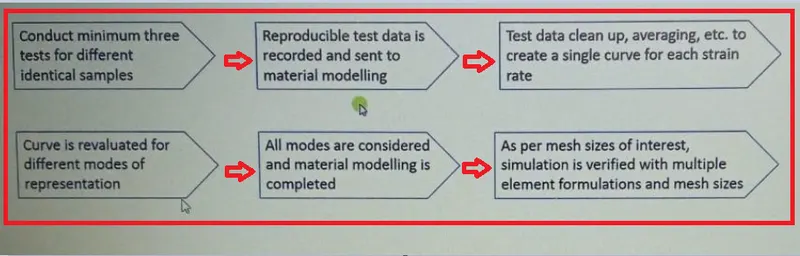
image source: Skill lync

Two points of verification

Parameters of verification (input data with results)

1. Modulus of Elasticity (E)
2. Engineering yield stress 0
3. Engineering ultimate stress
4. Elongation at failure
5. Reduction in area

Plot a simulation result with experimental data, if you given a input and if it is not working as input then definitely there is some problem in our model, so we need to check results with our input values.

Parameter of verification (results with test)

1. Different pattern on location: When part is failed, these points need to match, we can’t match with 100% but if you match up to 80 to 90% that is fine.
2. Load deformation plot
3. Location of stress strain value

Factor need to consider while modelling a material card

• Required accuracy
• Model complexity
• Solver ability
• Computational cost

Workflow of Material Modelling

• Extract the data from the diagram
• Clean the data and visually confirms that it matches the original data
• Convert the data to Kg mm ms unit system
• Process the data and create the material as demonstrated
• Use the material model as per dog-bone specimen and validate the same

Step 1: Extraction of Data

The data digitizer tool is used to extract the data from curve of the image shown below

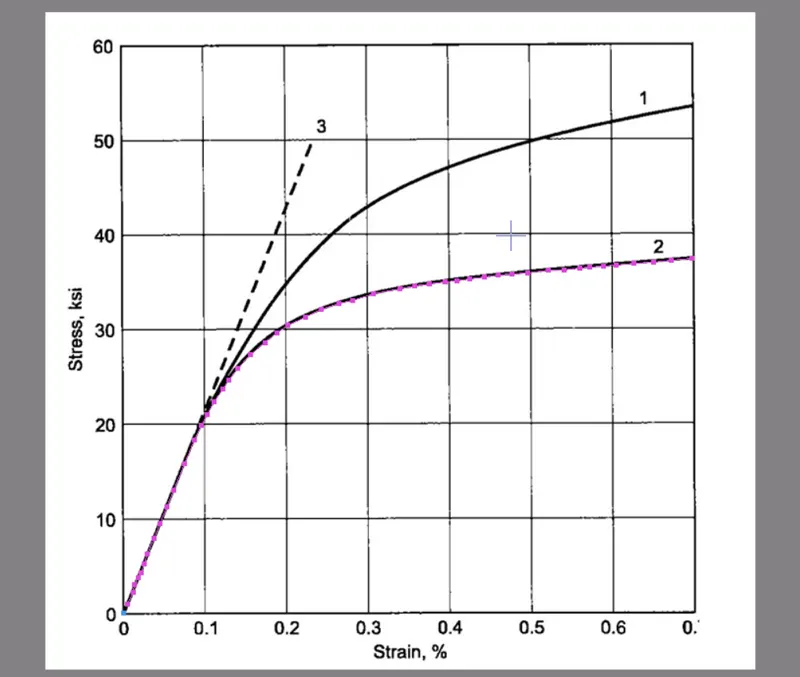
Here we extract the data points out from this curve by using tool

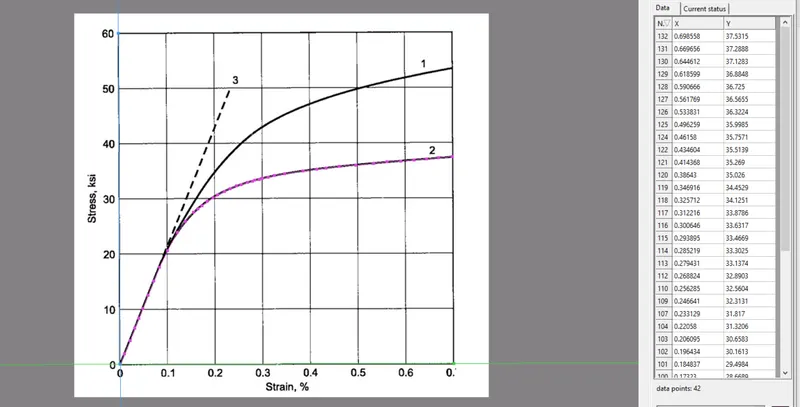
Extracted data points from the curve

After extracting data point from the curve, which is true stress – strain value are exported to an excel sheet, and values of true stress and strain are plotted.

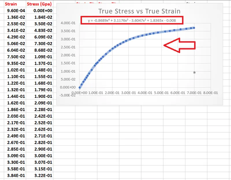
Curve Fitting

Here we have stress value in pound square per inch and the value of strain is given in percentage, so we have to convert the stress from psi to Gpa as per our unit system that we followed, after that we have to convert true strain into effective plastic strain.

Effective plastic Strain = Total true strain – True stress / E

Where E is Modulus of Elasticity which is 141.10

Effective stress is a true stress

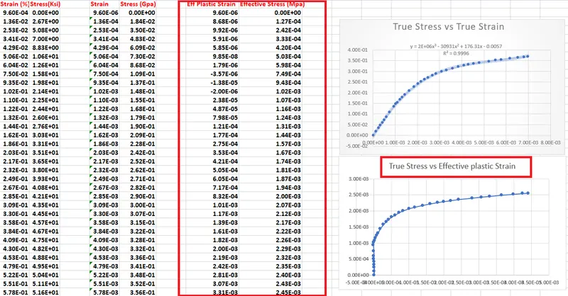
Effective Stress vs Effective plastic Strain

Here we have also do a curve fitting, to capture the curve mathematically, basically curve fitting is the process of constructing a curve, or mathematical function, that has best fit to a series of data point.

Fitted curve can be used as an aid for data visualization, to conclude values of function, where no data are available and to summarize the relationship among two or more variables.

Now after that we have to remove the elastic portion from the data set, because in Ls dyna, to define the elastic portion the value of E is only necessary, which is basically a slope of linear part, so only non-linear part needs to defined, we start our non-linear part from 0 because we subtract all the strain value from the elastic strain, so that it doesn’t taken into account, we subtract all the value from the strain up to yield point, that’s why our curve is starting from the 0 point.

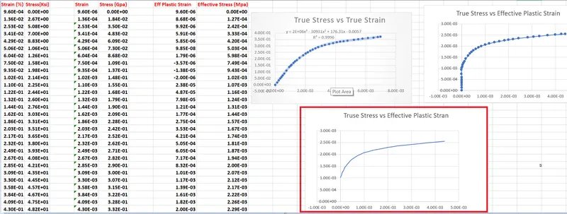
Nonlinear portion is defined

Now our material data is ready for define the nonlinear portion, and we have to define in the material model card (MAT_024), before defining the Material card and setup the simulation few things need to know before defining the MAT_024

MAT_024 is based on J2 Plasticity also popular as von-misses plasticity model

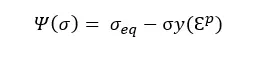
Ψ is yield function

σeq is a equivalent stress

σy is a yield stress which is function of plastic strain

Plastic strain is equivalent plastic strain, which is accumulated throughout the deformation processes, and basically what MAT_024 does or any J2 based plasticity algorithm, it check first if yield function is satisfied or not, and if for any instance, if the equivalent stress is bigger than the current yield stress then we have to use this algorithm in order to calculate, how much that deformation is plastic and how much is elastic. So if we plot this yield function in principle stress space (Cylindrical space), and this is a good thing of MAT_024 and J2 based plasticity model, because we don’t have any sharp corner, that might gives us bad derivative, one of the reason why MAT_024 is so efficient and so robust.

Flow rule, which basically tell us how much plasticity you have in that deformation state and is given as above

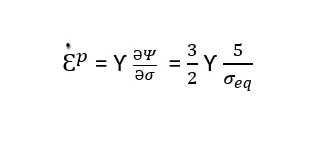
Ep= Plastic strain tensor in its rate

Ƴ = Plastic multiplier

So in case of Von misses model or MAT_024 this derivative is actually quite simple, so that’s the expression for the flow rule of MAT_024

This expression is quite simple in comparison to other model, sometimes user want to do more sophisticated model, for instance they just add some other dependency here in the huge function, and the result is that the function becomes more complicated, because of increase in derivative complexity, sometimes make a small change in yield function will lead to affect the flow rule, quite dramatically.

MAT_024 there is no rate dependence for numerical algorithm, in case of no strain rate dependent the plastic strain increment can be easily calculated, in case of viscoelasticity an iterative procedure is necessary, in order to find the solution of elasto-plastic problem.

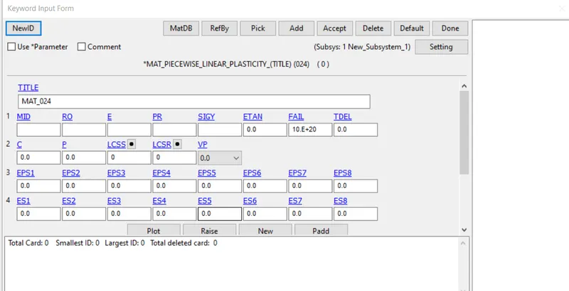
MAT_024 material card

FAIL Flag : This gives us option to define failure strain which is equivalent plastic strain at failure, most of user use this for general failure description, it’s something that is not recommendable to use this generally because failure strain is same for all possible stress state, we have same failure strain for tension and compression, which we know it’s not true. Keep in mind that when we use that failure criterion, it is very simple failure criterion and if you need a little more sophisticated, or a little more plastic, then we have to go for some other criteria or same criteria with damage model.

CP, P, LCSR all these flags are related to strain rate effects

CP is called Copper simons parameters used to define the effect of strain rate

LCSR is a curve that you can define, where you have scaling factors as a function of strain curve and we can multiply our plot with these scaling factors, to get different plots for different strain rates.

VP flag stands for visco-plasticity, used for defining the visco-plasticity effect

Defining the curve by EPS and ES values is generally not recommended, it is better to don’t use this, instead of that use load curve (which is much more better option)

So how can we defining the hardening, the easiest way is by using a single load curve or tables, curve which is plotted will interpolate linearly, that is the reason to call it piecewise, here between two points LS Dyna will always linearly interpolate, So the quality of our curve will depends upon the resolution of the curve, better to have more points for better resolution, there is no limit in defining the points, but only limitation is your hardware, so you need to have require enough memory for using all these points.

Strain rate effects:

There is different way of doing this, in ls dyna two things need to take care, 1^st thing is how to introduce the effect of strain rate and what is the information about the strain rate effect, the other thing is what is the formulation you want to use to considered those effects, so there are two separate things, sometimes it is little bit confused.

If you want to consider this dependency of strain rate well there are different ways

One way using this so called copper simons parameters (C&P), these parameter which are governed by the equation, and the equation is also a function of strain rate and what you have here is scaling factor, and this scaling factor will scale your yield curve depending on the strain rate.

Using (C&P) parameter, this idea is quite old actually, now days we can use better solution which are tables, we can use table to define the strain rate dependence. We can use exactly the same fag here as we did for single hardening curve with the difference is that we have several hardening curve for different strain rates. It gives us more flexibility to define different hardening curves for different strain rates.

Table solution (Curve) is the most practical or flexible one to define the strain rate effect in MAT_024

This is how we can define dependency, that is what is the effect of strain rates, what is the effect I am waiting or expecting and then we have VP flags that tells you about how to use that information to introduce the effect of strain rate.

Defining a table and curve in MAT_024 (MAT_PIECEWISE_LINEAR_PLASTICITY)

In the direction of plastic strain we have linear interpolation between he two points, the jump from one plastic strain to the another is very small, well in strain rate direction we have basically two option in LS-Dyna, we can either interpolate linearly or interpolate logarithmically, we have both the option.

If we want to do linear interpolation all we have to do just use MAT_PIECEWISE_LINEAR_PLASTICITY, we can define our tables with real stress strain value.

If you want to work with logarithmic interpolation, then there are two ways, one is defining your data logarithmically, means defining the value logarithmically, for small strains, we have negative values, and the other method is to use MAT_PIECEWISE-LINEAR_PLASTICITY_LOG_INTERPOLTION

Ls-dyna will interpolate the data in logarithmic manner, here we don’t need to define the logarithmic value, we can put direct values of effective stress and effective plastic strain and Ls-Dyna will calculate that accordingly.

*DEFINE CURVE & DEFINE TABLES

Generally in LS-DYNA when we defines the curve, these curves are internally re-discretized in LS-Dyna , by default the number of equally spaced intervals used in the re-discretization can be defined through the flag LCINT of the Keyword CONTROL_SOLUTION.

By default LCINT is set to 100 but it is recommended to increase this value in order to avoid loosing resolution of the input curve.

*CONTROL_OUTPUT

Sometimes you want to be sure that what ls-dyna using in my simulation, because I have use this re-discretization, I want to see that what it’s really using, there is a way of doing this, here in Control output we have flag called IP curve, we can switch this to one, LS-DYNA will output all the discretize curves in your d3Hsp file, it can be helpful in order to evaluate or asses if your curve has been re-discretize well or not, well discretization means is the re-discretization still similar to your original curve, sometimes it might change your curve, that you don’t want, so the way of debugging this by using this feature of LS-DYNA (IP Curve) in *CONTROL_OUTPUT

*DEFINE_CURVE

After we defined our curve up to certain limit, and if ls-dyna require data sets or points after that, then it simply extrapolate the curve linearly from taking reference or slope of last two points, that they are formed during re-discretization.

Model Setup in LS Dyna

Model import and Boundary conditions

The given dogbone specimen is imported into ls dyna, this only contain the nodes and elements, rest of thing we have to defined in order to conduct the test.

SPC

The boundary conditions are defined in such a way that it mimic the behavior of real situations

The node on the left edge of the specimen are constrained in the x direction and z direction, they are not constrained in the y direction, since the specimen undergoes lateral deformation during the test.

We took center node and constrained in the y direction.

MAT_024 / *MAT_PIECEWISE_LINEAR_PLASTICITY

Final remarks

• Work horse in crash simulation (very fast)
• Available for shell solid beam etc….
• No kinematic hardening is considered (*MAT_225 is similar to the *MAT_024 but allows additionally the definition of kinematic hardening)
• Unless visco-plasticity (i.e. VP =1) is activated, the plasticity routine doesn’t iterate, work very well in explicit, possibly problematic for large time step in implicit

HINT set IACC =1 in *CONTROL_ACCURACY in order to make *MAT_024 always iterate.

• The points between the rate dependent curves in a table are interpolated either linearly or logarithmically.
• The load curve are extrapolated in the direction of plastic strain by using the last slope of the curve
• Negative slopes are permitted but should generally avoided

Use Monotonically increasing curve gives you more numerical robustness in your model.

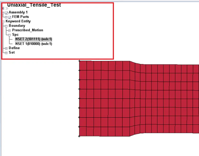
Defining constrained to the node

Prescribed motion

A displacement is given to the node at the right edge of the specimen as shown below

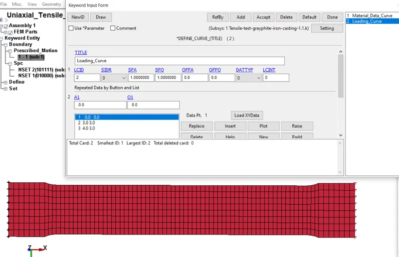
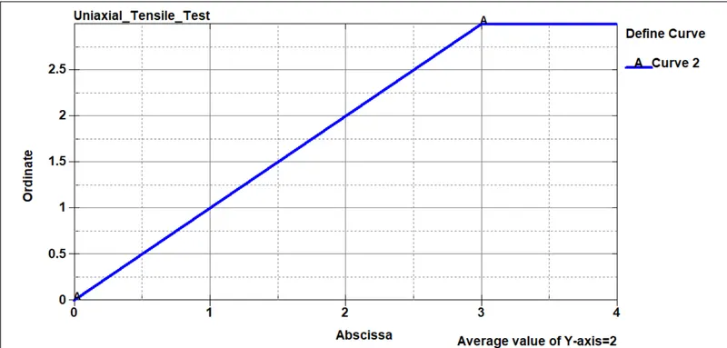
Defining loading condition

Material Card Definition

The MAT_024 piecewise linear card is defined with the following parameters, the unit system used is Kg-mm-ms. The Youngs modulus (E) is 2.09E+06 psi which is 144.10 Gpa, the value of density and poissons ration are defined accordingly.

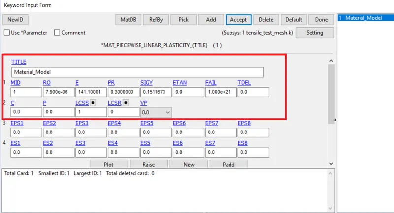
The LCSS contains the load curve of effective plastic strain and the effective (true) stress. The effective plastic strain is calculated in the excel sheet from the true strain and stress value using the relation

Effective plastic strain = True strain – (True stress / E)

The region of the curve after the yield point (141 Gpa) is the plastic part of the curve, which we defined in the Material card.

Material card is defined in ls-dyna

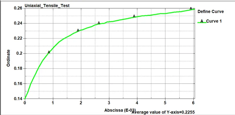
Defining Non-linear portion of the curve

Defining Element formulation / Section to the part

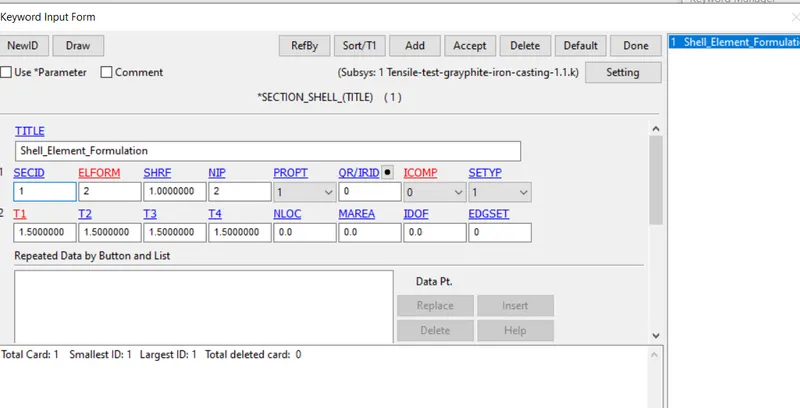
Part definition

The material and the section ID are then assigned to the dogbone specimen as shown below

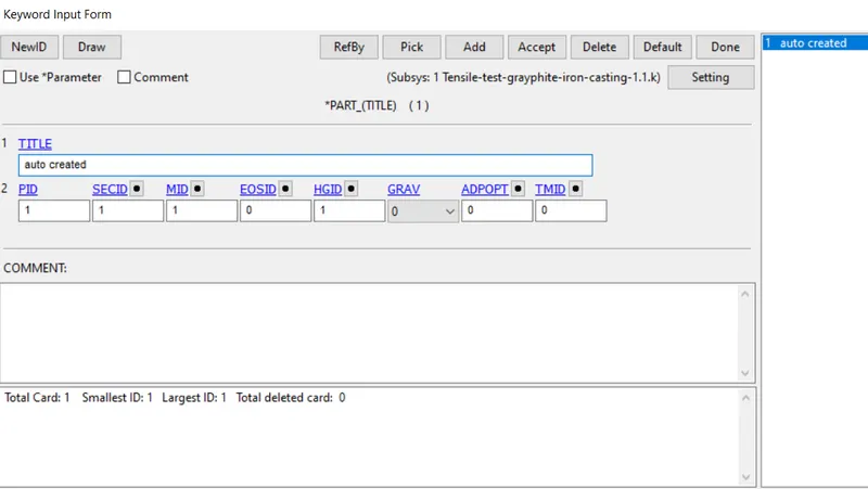
Assigning Section and Material ID to the Part

Database and Control cards

The database cards are defined as shown below.

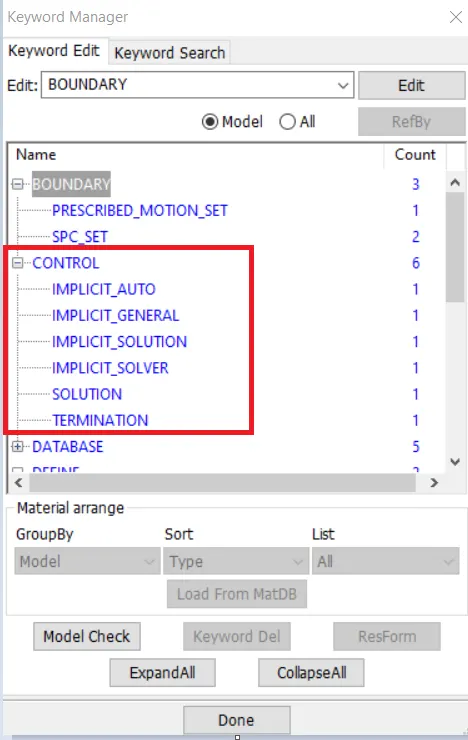
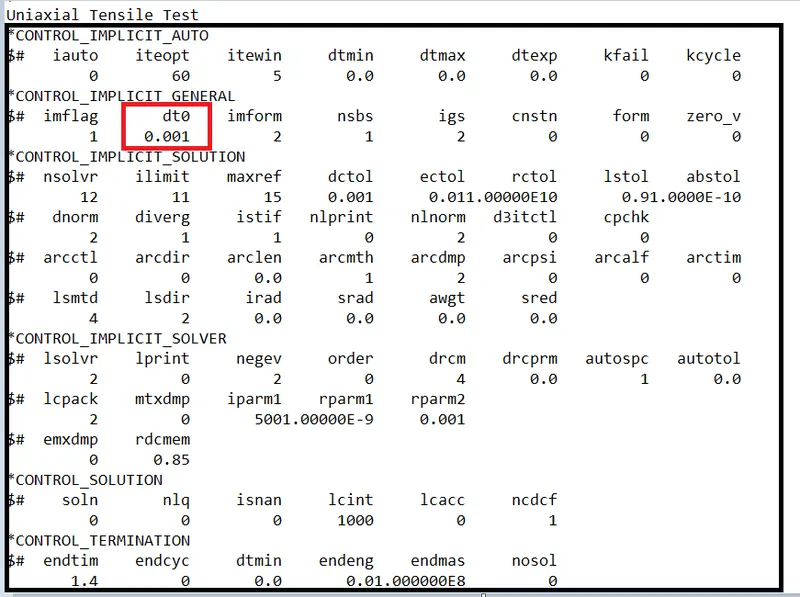
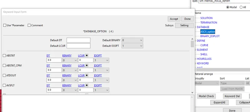
Controls and Database cards

Results and Conclusion

The model is simulated and the results are discussed below

Effective Plastic Strain

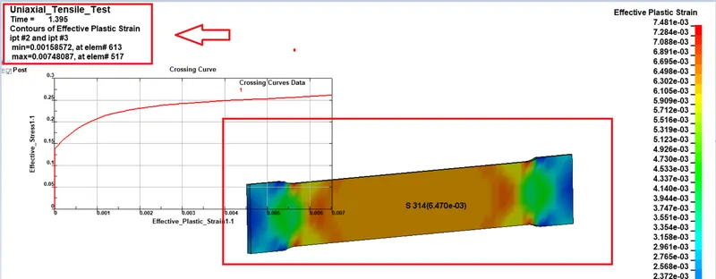
The Peak effective plastic strain is 0.00756

Effective Stress

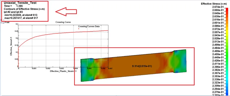
The peak effective stress is 0.267Gpa

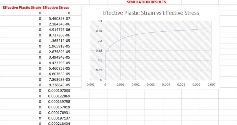
Simulation results

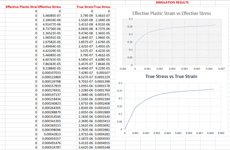
Simulation results (True stress vs True strain)

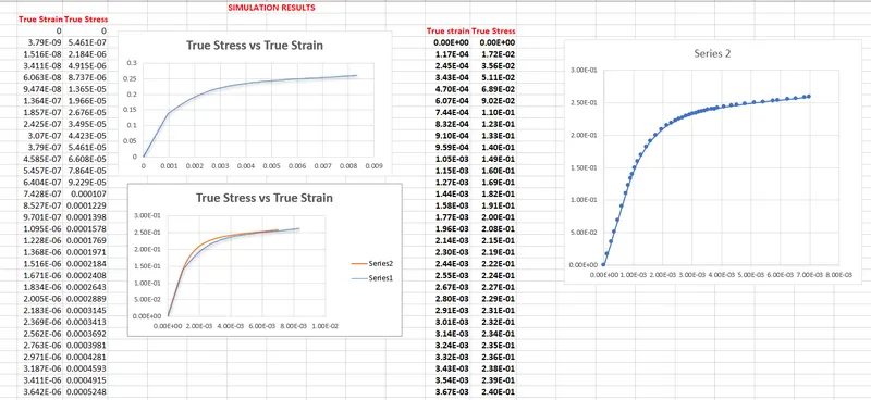
The curve we have obtain almost fits with the experimental data, but we have to do a improvement in them for getting more accurate results, thus the given values are verified and validated using the MAT_024 material card (Input data with the results), also we have another parameter of verification (result with test), where we compare the deformation pattern, load deformation plot, and location of stress strain value.

Hence, we were able to model a Material card using the stress strain data extracted from the given input, and we successfully verified it by comparing with the input results, but we also have to do other sets of verification and validations, we can check it at component level or may be at sub-assembly level, also we have to try up with the number of material cards with different mesh sizes element formulation, Hourglass effects needs to taken out for proper validation of material model.