Week 9 - FVM Literature Review

The Finite volume method :

Need for the finite volume method :

The finite difference schemes are limited in their ability to compute the property value when the geometry is irregular. An irregular geometry when meshed, has the irregular shaped individual elements. Calculation of the property value at the nodes becomes difficult and sometimes might not even be feasible.

This calls for the finite volume method which calculates the property value at the centroid of the individual volume called "cell". Thus the benefit it has is, irrespective of the shape of the mesh the discretized governing equations are still used.

The use of the unstructured meshes which occur in most cases is the main advantage of FVM. For the same number of elements, the mesh can be strategically constructed to give the optimum result.This allows to capture phenomena like shock waves and boundary layer effects which occur only at only certain geometric location.

The Finite Volume approach to solving the governing equations:

The Finite Volume method (FVM) is a method for representing and evaluating the PDE in the form of algebraic equations. In this method, the volume integral in a PDE that contain a divergence term are converted to surface integrals, using the divegence theorem. These terms are evaluated as fluxes at the surfaces of each finite volume.

A general principle on which FVM is based is that flux entering a given volume is equal to the sum of the flux leaving the same control volume and the remains of the flux in the volume.

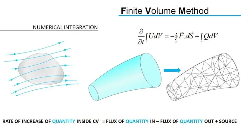
The conservation law :

The variation of the conserved flow quantity within a given volume is due to the net effect of some internal sources and the amount of quantity which is crossing the boundary surface.

General form of the conservation law :

`(delU)/(delT)*int_V(U dV) + int_svec(F) *vec(ds) = int_v(Q)dV`

The term `(delU)/(delT)*int_V(U dV)`represents the variation of the flow quantity and `int_svec(F) *vec(ds)`represents the flux crossing a suface with surface area ds.

The need for the interpolation schemes :

The finite volume method provides the values of the property at the centroid of a cell. The approximation of surface integrals and volume integrals may require the value of the variable at locations other than those at centroid and can be obtained by interpolation.

The most popular interpolation schemes in FVM are [1]:

1. Upwind scheme :

The UDS for approximation of the value of the variable at the east of the face of a Control volume is given by :

`f_e = [[fp if v.n_e > 0],[f_E if v.n_e < 0]].`

• The upwind scheme is equivalent to using the forward or backward finite difference approximation.
• The upwind scheme is first order accurate and is associated with the numerical diffusion `Gamma_(e) = (rho*u)_e * (Deltax)/(2)`

2. Linear interpolation :

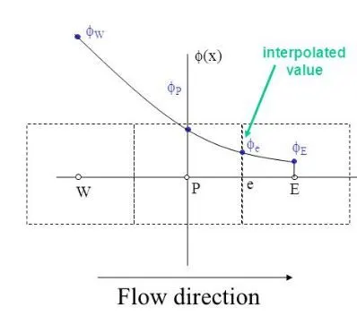
As per the linear interpolation, the approximate value of the property/ variable at the face center can be found by the linear interpolation of variables at two nearest computational nodes.

Hence at e;

`f_e = f_E*lambda_e + f_p *(1 - lambda_e)`

Here, `lambda = (x_e - x_p)/(x_E - x_p)`

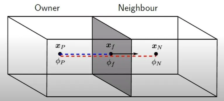
• Linear interpolation is equivalent to the central difference scheme and is second order accurate.

3. Quadratic upwind interpolation (QUICK)

As per the QUICK,

`phi_e = 6/8*(phi_U) + 3/8*(phi_D) - 1/8*(phi_(UU))`

D represents the downstream cell.

U represents the upstream cell.

UU represents the second upstream cell.

Flux limiters [2]:

Flux limiters are used in numerical schemes for solving the problems of fluid dynamics, described by the highly coupled non linear PDE. The main intention behind using the flux limiters is to limit the spatial derivative terms near the dicontinuities to the physical real values. They come in handy when sharp waves / peaks are present.

The main sourece of oscillations/ peaks is because of the extrapolation. When extrapolation is performed there is a chance of overshooting or undershooting.

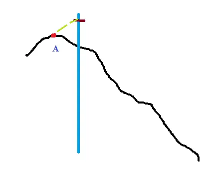
Suppose we were to determine the variable value at the location where the intersection of the line and curve, the easy way to do is to extrapolate the variable value at A to the point on the straight line. That's where the accuracy is lost and the oscillations set in.

References :

1. Lecture 18, Finite volume interpolation schemes, NPTEL-IIT Roorkee.http://150.107.117.36/NPTEL_DISK4/NPTEL_Contents/Web_courses/Phase2_web/112107080/module4/lecture3/lecture3.pdf

2. Flux limiters : Lecture by Qiqi wong. https://www.youtube.com/watch?v=Wtx50YanRnw