Week 9 - FVM Literature Review
To describe Finite volume method
Introduction:
Finite volume Method:
The finite volume method (FVM) is a method for representing and evaluating partial differential equations in the form of algebraic equations. In the finite volume method, volume integrals in a partial differential equation that contain a divergence term are converted to suraface integral, using the divergence theorem. These terms are then evaluated as fluxes at the surfaces of each finite volume. Because the flux entering a given volume is identical to that leaving the adjacent volume, these methods are conservative.
Finite Difference Method:
In numerical analysis, finite-difference methods (FDM) are a class of numerical techniques for solving differential equations by approximating derivatives with finite differences. Both the spatial domain and time interval (if applicable) are discretised, or broken into a finite number of steps, and the value of the solution at these discrete points is approximated by solving algebraic equations containing finite differences and values from nearby points.
Finite difference methods convert ordinary differential equation (ODE) or partial differential equation(PDE), which may be nonlinear, into a system of linear equations that can be solved by matrix algebra techniques. Modern computers can perform these linear algebra computations efficiently which, along with their relative ease of implementation, has led to the widespread use of FDM in modern numerical analysis.Today, FDM are one of the most common approaches to the numerical solution of PDE, along with finite element method.
The major Differences include:
differences in defination:
Finite Difference method:
The finite-difference method is the most direct approach to discretizing partial differential equations. You consider a point in space where you take the continuum representation of the equations and replace it with a set of discrete equations, called finite-difference equations. The finite-difference method is typically defined on a regular grid and this fact can be used for very efficient solution methods. The method is therefore not usually used for irregular CAD geometries, but more often for rectangular or block-shaped models.
There is a connection with the finite-element method: Certain formulations of the finite-element method defined on a regular grid are identical to a finite-difference method on the same grid. Regular grids can often be used in meteorological, seismological, and astrophysical simulations, for example.
Finite Volume Method:
The finite-volume method is similar to the finite-element method in that the CAD model is first divided into very small but finite-sized elements of geometrically simple shapes. Apart from this, the finite-volume method is very different from the finite-element method, beginning with the concept of elements, which are instead referred to as cells.
The finite-volume method is based on the fact that many physical laws are conservation laws—what goes into one cell on one side needs to leave the same cell on another side. Following this idea, you end up with a formulation that consists of flux conservation equations defined in an averaged sense over the cells. Historically, this method has been very successful in solving fluid flow problems
The major difference may be included as :
Each method is quite similar in that it represents a systematic numerical method for solving PDEs. One important difference is the ease of implementation. A common opinion is that the finite-difference method is the easiest to implement and the finite volume method is difficult comparitively. One reason for this may be that the finite-volume method requires quite sophisticated mathematics for its formulation.
The Advantages and Disadvantages of Finite Difference method:
The finite-difference method is defined dimension per dimension; this makes it easy to increase the “element order” to get higher-order accuracy. If you can fit the simulation in a rectangular or box-shaped geometry using a regular grid, efficient implementations are much easier than for finite-element and finite-volume methods. Regular grids are useful for very-large-scale simulations on supercomputers often used in, as mentioned before, meteorological, seismological, and astrophysical simulations.
With the finite-difference method, you may easily run into problems handling curved boundaries for the purpose of defining the boundary conditions. Boundary conditions are needed to truncate the computational domain. They represent communication with the surrounding world, which is the part that you do not want included in your simulation. If one can overcome the boundary-condition problem on curved boundaries, the method gives very efficient and high quality results.
For computations that need high accuracy, the extra effort in making boundary-fitted meshes and the associated complications of such meshes for the implementation may be worth it. Examples include Formula 1 car computational-fluid-dynamic (CFD) simulations and space-shuttle CFD simulations. The finite-difference method is more difficult to use for handling material discontinuities. In addition, it does not lend itself for local grid refinement or anything similar to “adaptive mesh refinement.” This may be needed to resolve local rapid variations in solutions such as around a corner of a complex shape, as described earlier.
The Advantages and Disadvantages of Finite Volume method:
The finite-volume method is a natural choice for CFD problems, since the partial differential equations you have to solve for CFD are conservation laws. However, both finite differences and finite elements can also be used for CFD. Efficient technology for CFD with the finite-element method has become increasingly popular over the last 10 to 15 years. Techniques for CFD with the finite-difference and finite-volume method have been known and used much longer.
The finite-volume method’s strength is that it only needs to do flux evaluation for the cell boundaries. This also holds for nonlinear problems, which makes it extra powerful for robust handling of (nonlinear) conservation laws appearing in transport problems.
The local accuracy of the finite-volume method, such as close to a corner of interest, can be increased by refining the mesh around that corner, similar to the finite-element method. However, the functions that approximate the solution when using the finite-volume method cannot be easily made of higher order. This is a disadvantage of the finite-volume method compared to the finite-difference methods.We cannot use it directly ,when the grids are not aligned along x,y or z direction.For example if we consider a plane
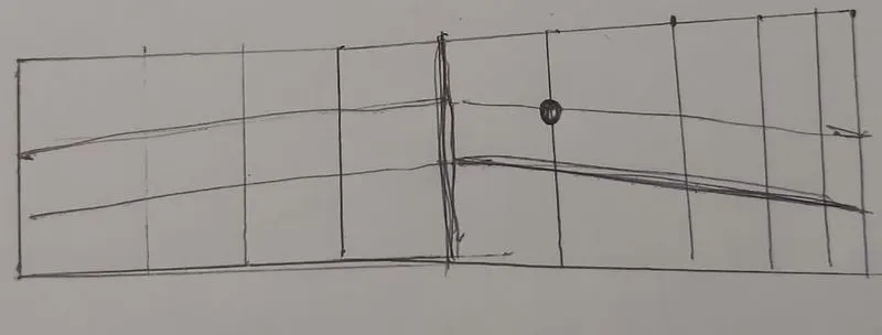
We could see that the grids are not properly aligned due to which we cannot solve any differential equations with with this kind of mesh as we do not get the next mesh point.We have to include some correction terms.This process become extremely tedious.We can overcome this by variable tranformation approach.The variable transformation approach
we can create a variable space .In eeta and epslon space the grid looks similar to that of the cartesian form.Sutiable mapping fucntion are defined so they synchronize two functions at two different planes.This is pretty tough job to convert tranformstion from one grid form to other.
Some of the examples of Finite Difference method:
Weather calculations, astrophysics, seismology, physical realism in computer graphics, and special effects.
Some of the examples Finite Volume method:
CFD, heat transfer, and chemical engineering
In FVM method instead of writing equation for a single point ,we write equations for an entire volume.Also for a considered volume no assumptions are made over the shape of the volume .Inside this particular volume the flow is conserved ,flow quantities are conserved ,energy ,mass ,momentum is conserved and so on .This is called Finite volume Representation .The starting point of FVM is with integral form of governing equations.
Some of the steps of Finite volume descretisations includes:
- Wrting the required governing equations.
- Applying Gauss Divergence theorem.
- We obtain discretised form which can be solved digitally.
Considering the 1 D steady state heat conduction equation along with the source.
`(del(alpha*(delT)/(delx)))/(delx) +S = 0`
The above is the governing equation or the conservation equation.This is valid at every point in the domain whic means it is valid in entire control volume.
Where
S is the source term.
`alpha` is the thermal diffusivity term.
`(delT)/(delx)` is the temperature Gradient along x direction.
The diagramatic representaion for this include:or may be called Finite volume representation.
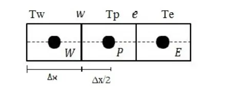
Now if we consider a control volume `dv` andf it is multiplied with the above equation and integrated for entire volume then it should be equal to 0 .Which is the integral form of the governing equation.
if we validata at a single point it s valid at all the points in the contol volume `dv`.
Multiplying the equation by dv we get,
`=>int((del(alpha*(delT)/(delx)))/(delx) +S )dv = 0`
`=>int((del(alpha*(delT)/(delx)))/(delx) )dv+intS dv = 0`
Also we know that `dv=Adx`
`=>int((del(alpha*(delT)/(delx)))/(delx))A*dx +intS dv = 0`
`=>[alpha*A*(delT)/(delx)]_w^e +barS*dv = 0`
here `barS` is the average of the quantity S as we replace it by avearge term mulitplied by dv which will be giving the area under the graph of S vs x which is same as `intS*dv`.
if we assume `alpha` as a constant and not as a function of temperature then,
`alpha*A*[(T_e-T_p)/(Deltax)]-alpha*A*[(T_p-T_w)/(Deltax)]+barS*dv = 0`
Now if the source term is the function of temperature we have to linearize it.also we have to linearize the`alpha`as well as it is the fucntion of temperature we have to linearize it as well.
`S_("linearization") -> S_u + S_p*T_p`
`underbrace(alpha*A*[(T_e-T_p)/(Deltax)])_((heat flux )_(out))-underbrace(alpha*A*[(T_p-T_w)/(Deltax)])_((heat flux)_("in"))+underbrace(barS*dv )_("soucrce term")= 0`
The amount of heat rmeoved from a particular box is conserved.
Gradient Schemes:
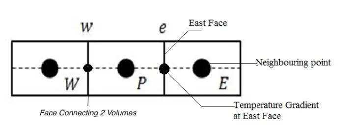
From the above diagramatic representation when we calculate temperature gradient on east face we basically use temperature from the neighbouring point trying to evaluate or numerically represent gradient of temeperature which is called as gradient scheme.
Interploation Schemes
The approximations of surface and volume integrals require values of the variable at location other than the computational nodes of the cotrol volume .Vlaues at these locations are obtained using the interpolation formulas.
Some interploation methods include:
- Upwind interploation
- Linear Interpolation
- Quadratic upwind interploation.
- Hybrid ,TVD and ENO interpolation schemes.
Lets consider example of one dimensional convection and diffusion.
`(d(rho*u*phi))/(dx) = (d/dx(tau*(dphi)/(dx)))`
Where `phi` is the solution variable (scalar)
`rho` is the density ,`u` is the velocity ,`tau` is the diffusion coefficient.Similar to the FVM representaion we can dicertize it into three blocks which yields the following
`(rho*u*phi)_e-(rho*u*phi)_w = (tau*(dphi)/(dx))_e-(tau*(dphi)/(dx))_w`
1) Upwind interploation (UDS)
This schemes takes into count that the direction of fluid flow and based on it the value of solution variable at the face is approximated by its value at the upstream computational node.For example if fluid would have moved from west to east then
`phieapproxphiP`
if the fluid moving from the east to west then
`phi_e = phiE`
2) Linear interploation scheme
Inorder to approximate the value of variable at control volume face center by two nearest computational nodes location e.This is equivalent to a central differencind scheme of first order derivative .It is second order accurate and produce oscillatory solutions.The relation for linear interpolation is as follows:
`f_e = f_E*lamda_e +f_p*(1-lambda_e)`
where `lamda_e = (x_e -x_p)/(x_E-x_P)`
3)Hybrid interploation scheme: It is the blend of UDS and CDS .The hybrid difference scheme exploits the favourable properties of the upwind and central differencing schemes.It switches to upwind and central differencing schemes.It switches to upwind differencing when central differencing produces inaccurate results at high Pe number.The scheme is fully conservative and since the coefficients are always positive it is unconditionally bounded .It satisfies the transpotiveness requirement by using upwind formulation for large values of Peclet Number
`f_e =gamma*f_("CDS")+(1-gamma)*f_("CDS")`
4)QUICK scheme:
In computational fluid dynamics QUICK, which stands for Quadratic Upstream Interpolation for Convective Kinematics, is a higher-order differencing scheme that considers a three-point upstream weighted quadratic interpolation for the cell face values.
For the one-dimensional domain shown in the figure the Φ value at a contol volume face is approximated using three-point quadratic function passing through the two bracketing or surrounding nodes and one other node on upstream side.In the figure, in order to calculate the value of the property at the face, we should have three nodes i.e. two bracketing or surrounding nodes and one upstream node.
- Φw when uw > 0 and ue > 0 a quadratic fit through WW, W and P is used,
- Φe when uw > 0 and ue > 0 a quadratic fit through W, P and E is used,
- Φw when uw < 0 and ue < 0 values of W, P and E are used,
- Φe when uw < 0 and ue < 0 values of P, E and EE are used.
`f_e =f_E+g1*(f_D-f_U)+g2*(f_("UU")-f_("U"))`
where
`g1=((x_e-x_U)*(x_e-x_("UU")))/((x_("UU")-x_("U"))*(x_(UU)-x_(D))`
`g2=((x_e-x_U)*(x_e-x_("D")))/((x_("UU")-x_("U"))*(x_(UU)-x_(D))`
5)Total variation diminshing scheme(TVD)
TVD schemes are designed to address the undesirable oscillatory behaviour of higher oreder schemes.In TVD schemes the tendency towards oscillation is counteracted by adding an artificial diffusion fragment or by adding a weighted towards upstream contribution.
It is 2nd order accurate
`f_e=f_p+1/2*(psi(r)*(f_E-f_P)`
where `psi(r)` is the flux limiter fuction.
where ,
`r=(u_i-u_(i-1))/(u_(i+1)-u_i`
Flux Limiters:
For convective fluid flow ,it is ovserved that low order schemes are usually stable but quite dissipative in nature around the points of discontinuity or shocks while the higher order schemes are unstable in nature and show oscillations in the vicinity of discontinuity or shocks .Highly accurate and oscillations free schemes are known as High Resolution schemes.
In order to make the scheme TVD we must constrain or limit the range of possible values of the additional convective flux `f_e=f_p+1/2*(psi(r)*(f_E-f_P)` which was originally introduced to make the scheme high-order .Hence the function `psi(r)` is called a limiter function.
Flux limiter functions are used to fine tune the higher order and lower order schemes in such a way that the resulting scheme gives a higher order accuracy in the smooth region of the flow and maintains first order accuracy in the vicinity of shocks and discontinuities.For such a scheme TVD scheme is employed.
`F(u_(i+1/2)) = f^(low)(i+1/2)-psi(r_i)*(f^(low)(i+1/2)-f^(high)(i+1/2))`
`F(u_(i-1/2)) = f^(low)(i-1/2)-psi(r_i-1)*(f^(low)(i-1/2)-f^(high)(i-1/2))`
where
`f^(low)` is the low precision flux (of first oreder)
`f^(high)` is the high precision flux (higher order)
Conlusion :
We could say that the finite volume method is used exceptionally in cfd problems.It has its own domain of application where it is in tremendous usage.Even though it is difficult to code but gives an added advantage of its robustness.