Week 5 - Mid term project - Solving the steady and unsteady 2D heat conduction problem

THE MID TERM PROJECT SOLVING STEADY AND UNSTEADY 2D HEAT CONDUCTION

THEORY:The transfer of heat is usually called heat condurction.This is a quite intresting phenomenon to research with.

Heat equation:he heat equation is a certain partial differential equation. Solutions of the heat equation are sometimes known as caloric functions. The theory of the heat equation was first developed byjoesph Fourier in 1822 for the purpose of modeling how a quantity such as heat diffuses through a given region.

The heat equation can be given as follows:

this is for the 3-Dimensional general case.

`(delu)/(delt) = K*((del^2u)/(delx^2)+(del^2u)/(dely^2)+(del^2u)/(delz^2))`

where `K` is the coefficient called diffusivity.

The types of heat conduction:

• Steady-state conduction is the form of conduction that happens when the temperature difference(s) driving the conduction are constant, so that (after an equilibration time), the spatial distribution of temperatures (temperature field) in the conducting object does not change any further.
• Transient conduction:During any period in which temperatures changes in time at any place within an object, the mode of thermal energy flow is termed transient conduction.

Heat conduction in Steady state for 2-Dimension case:

The discrete spacing in x and y direction can be defined as dx,dy respectively.here is the derivation for descretisation,which could be used in our program.

`(T_(l)-2*T_p+T_r)/(delx^2)+(T_t-2*T_p+T_b)/(dely^2) = 0` -(1)

For SOR method it turns out to be a small change with the introduction of the relaxation factor.

`T_(ij)^(k+1)=T_(ij)^k*(1-omega)+omega*T_(gs)(i,j)`

where `T_(gs)` is the result of the Gauss Sidel method.

The diagramatic representation of the problem can be as follows:

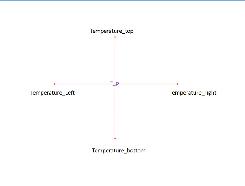
The equation 1 can be simplified as follows:

`2*(T_p/(delx^2)+T_p/(dely^2))=(T_l+T_r)/(delx^2)+(T_t+T_b)/(dely^2)`

`T_p*(2*(delx^2+dely^2)/(delx^2*dely^2))=RHS`

`K=2*[(delx^2+dely^2)/(delx^2*dely^2)]`

`T_p= 1/K*((T_l+T_r)/(delx^2)+(T_t+T_b)/(dely^2))` -(2)

Now suppose we assume

Our we just type as (2) our programming equation.

As far as the programming statement is concerned it will be

`T_(i,j) = 1/K*((T_(i-1,j)+T_(i+1,j))/(Deltax^2) + (T_(i,j-1)+T_(i,j+1))/(Deltay^2))`

THE CODE FOR JACOBI ITERATION

%implicit jacobi for steady state
close all
clear all
clc

nx = 11;
ny = nx;

x= linspace(0,1,nx);
y= linspace(0,1,ny);

dx = x(2)-x(1);
dy =dx;

error = 9e9;
tolerance = 1e-4;

Temperature_Left=400;
Temperature_Top = 600;
Temperature_Right=800;
Temprature_Bottom=900;

T=300*ones(nx,ny);

T(2:ny-1,1)=Temperature_Left;
T(2:ny-1,nx)=Temperature_Right;
T(1,2:nx-1)=Temperature_Top;
T(ny,2:nx-1)=Temprature_Bottom;

T(1,1) = (Temperature_Top+Temperature_Left)/2;
T(nx,ny) = (Temperature_Right+Temprature_Bottom)/2;
T(1,ny)=(Temperature_Top+Temperature_Right)/2;
T(nx,1)=(Temperature_Left+Temprature_Bottom)/2;
k= 2*(1/(dx^2)+1/(dy^2));

T_initial = T;
Temperature_old = T;

iterative_solver = 1;

%jacobi method
if iterative_solver == 1
    jacobi_iteration=1;
    while(error>tolerance)
        for i=2:nx-1
            for j=2:ny-1
                T(i,j) = (1/k)*((Temperature_old(i-1,j)+Temperature_old(i+1,j))/(dx^2)+(Temperature_old(i,j-1)+Temperature_old(i,j+1))/(dy^2));
            end
        end
        error = max(max(abs(Temperature_old - T)));
        Temperature_old = T;
        jacobi_iteration = jacobi_iteration + 1;
    end
end
%plotting
figure(1)
contour(x,y,T)
clabel(contourf(x,y,T))
colorbar
colormap
colormap(jet)
set(gca,'ydir','reverse')
xlabel('X-axis');
ylabel('Y-axis');
title(sprintf('No of iterations in jacobi method = %d',jacobi_iteration));
pause(0.03);

Algo for code :

• we define the initial parameters the total number of grid points in x and y axis.
• then we define the uniform distribution of grid points dx and dy.
• we would set the error as 9e9 and tolerance as 1e-4.
• As per the question we would define the Temeperature necessary as per question.
• we set the iterative methos such that it works for error>tolerance.we define the necessary condition such that this loopcan terminate.we set the equation 2 in the loop inorder to get the values of temperature according to jacobi method.
• we plot the contour and keep the count of iterations.along with setting of title and label etc.

PLOT FOR JACOBI METHOD.

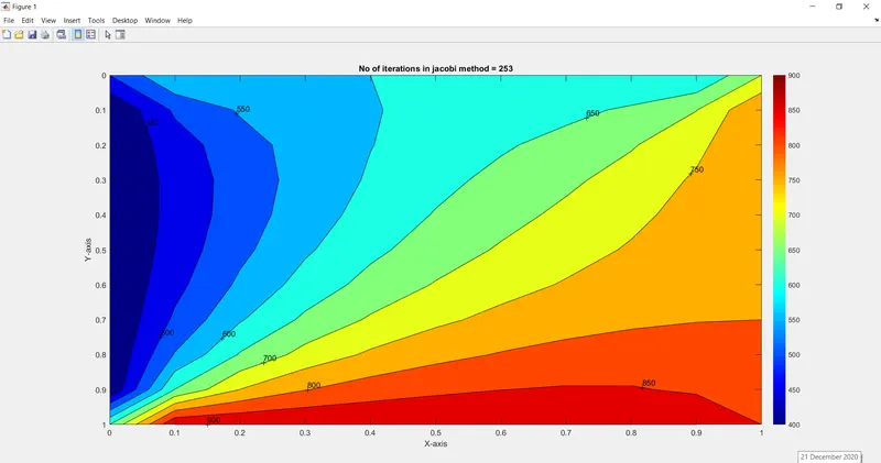
we could see the Wide range of contour with varying values.

THE CODE FOR GAUSS SIDEL METHOD

%implicit gausssidel for steady state
close all
clear all
clc

nx = 11;
ny = nx;

x= linspace(0,1,nx);
y= linspace(0,1,ny);

dx = x(2)-x(1);
dy =dx;

error = 9e9;
tolerance = 1e-4;

Temperature_Left=400;
Temperature_Top = 600;
Temperature_Right=800;
Temperature_Bottom=900;

T=300*ones(nx,ny);

T(2:ny-1,1)=Temperature_Left;
T(2:ny-1,nx)=Temperature_Right;
T(1,2:nx-1)=Temperature_Top;
T(ny,2:nx-1)=Temperature_Bottom;

T(1,1) = (Temperature_Top+Temperature_Left)/2;
T(nx,ny) = (Temperature_Right+Temperature_Bottom)/2;
T(1,ny)=(Temperature_Top+Temperature_Right)/2;
T(nx,1)=(Temperature_Left+Temperature_Bottom)/2;


T_initial = T;
Temeperature_old = T;

iterative_solver = 2;
k = 2*(1/(dx^2)+1/(dy^2));

%gauss sidel method
if iterative_solver == 2
    gauss_iteration=1;
    while(error>tolerance)
        for i=2:nx-1
            for j=2:ny-1
                T(i,j) = 1/k*((T(i-1,j)+Temeperature_old(i+1,j))/(dx^2)+(T(i,j-1)+Temeperature_old(i,j+1))/(dy^2));
            end
        end
        error = max(max(abs(Temeperature_old - T)));
        Temeperature_old = T;
        gauss_iteration = gauss_iteration + 1;
    end
end
%plotting
figure(1)
contour(x,y,T)
clabel(contourf(x,y,T))
colorbar
colormap
colormap(jet)
set(gca,'ydir','reverse')
xlabel('X-axis');
ylabel('Y-axis');
title(sprintf('No of iterations in Gauss sidel  method = %d',gauss_iteration));
pause(0.03);

Algo for code:

• we define the initial parameters the total number of grid points in x and y axis.
• then we define the uniform distribution of grid points dx and dy.
• we would set the error as 9e9 and tolerance as 1e-4.
• As per the question we would define the Temeperature necessary as per question.
• we set the iterative methos such that it works for error>tolerance.we define the necessary condition such that this loopcan terminate.we set the equation 2 in the loop inorder to get the values of temperature according to gauss method by applying the formula of the method.
• we plot the contour and keep the count of iterations.along with setting of title and label etc.

PLOT FOR GAUSS SIDEL

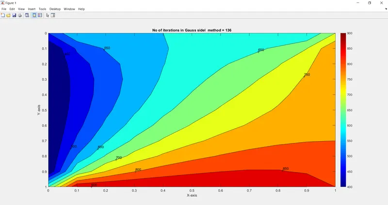
THE CODE FOR SOR METHOD

%implicit SOR  for steady state
close all
clear all
clc

nx = 11;
ny = nx;

x= linspace(0,1,nx);
y= linspace(0,1,ny);

dx = x(2)-x(1);
dy =dx;

error = 9e9;
tolerance = 1e-4;
omega = 1.2;



T=300*ones(nx,ny);

Temperature_Left=400;
Temperature_Top = 600;
Temperature_Right=800;
Temperature_Bottom=900;

T(2:ny-1,1)=Temperature_Left;
T(2:ny-1,nx)=Temperature_Right;
T(1,2:nx-1)=Temperature_Top;
T(ny,2:nx-1)=Temperature_Bottom;

T(1,1) = (Temperature_Top+Temperature_Left)/2;
T(nx,ny) = (Temperature_Right+Temperature_Bottom)/2;
T(1,ny)=(Temperature_Top+Temperature_Right)/2;
T(nx,1)=(Temperature_Left+Temperature_Bottom)/2;


T_initial = T;
T_old = T;
k=2*(1/dx^2+1/dy^2);

iterative_solver = 3;

%succesive over relaxation method
if iterative_solver == 3
    SOR_iteration=1;
    while(error>tolerance)
        for i=2:nx-1
            for j=2:ny-1
                T(i,j) = omega*(1/k*((T(i-1,j)+T_old(i+1,j))/(dx^2)+(T(i,j-1)+T_old(i,j+1))/(dy^2)))+(1-omega)*T_old(i,j);
            end
        end
        error = max(max(abs(T_old - T)));
        T_old = T;
        SOR_iteration = SOR_iteration + 1;
    end
end
%plotting
figure(1)
contour(x,y,T)
clabel(contourf(x,y,T))
colorbar
colormap
colormap(jet)
set(gca,'ydir','reverse')
xlabel('X-axis');
ylabel('Y-axis');
title(sprintf('No of iterations in SOR  method = %d',SOR_iteration));
pause(0.03);

Algo for code:

• we define the initial parameters the total number of grid points in x and y axis.
• then we define the uniform distribution of grid points dx and dy.
• we would set the error as 9e9 and tolerance as 1e-4.
• As per the question we would define the Temeperature necessary as per question.
• we set the iterative methos such that it works for error>tolerance.we define the necessary condition such that this loopcan terminate.we set the equation 2 in the loop inorder to get the values of temperature according to SOR method by applying the formula.
• we plot the contour and keep the count of iterations.along with setting of title and label etc.

THE PLOT FOR SOR METHOD

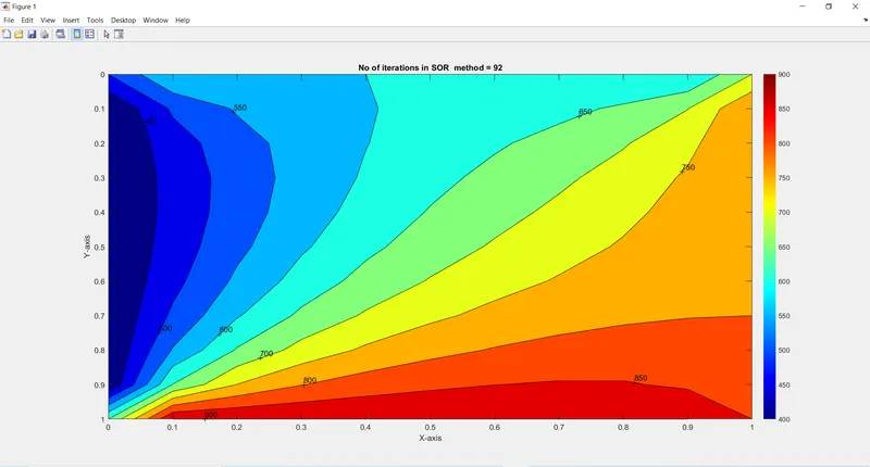
conclusion from above :

• The number of iteration for SOR is 92 ,jacobi is 253 and Gauss sidel is 136 which means least for SOR method.
• The convergence rate in case of steady state is faster in all the three methods,generally.
• These are the conclusions drawn from the plots above.

TRANSIENT STATE HEAT CONDUCTION

If the temperature of the body varies at any point with time as well as position then its the transient heat conduction.

The 2-D formula for heat conduction can be given as follows:

`(delT)/(delt) = alpha*((del^2T)/(delx^2)+(del^2T)/(dely^2))`

`(T_p^(n+1) - T_p^n)/(delt)= alpha*((T_l-2*T_p+T_r)/(delx^2)+(T_t-2*T_p+T_b)/(dely^2))^(n or n+1)`

`k1=alpha*((delt)/(delx^2))`

`k2=alpha*((delt)/(dely^2))`

here n is for explicit method.

and n+1 for implicit method.

The final equation would be,

For explicit method

`T_p^(n+1) = T_p^(n) + k1*(T_l-2*T_p+T_r)^n + k2*(T_t- 2*T_p+T_b)^n` -(3)

For implicit method

`T_p^(n+1) = 1/(1+2k1+2*k2)*(T_p^(n) + k1*(T_l+T_r)^(n+1)+k2*(T_t+T_b)^(n+1))` -(4)

%Transient analysis  explicit
close all
clear all
clc

nx=10;
ny=nx;
nt=1400;
x=linspace(0,1,nx);
y=linspace(0,1,ny);

dx=x(2)-x(1);
dy=dx;
error= 9e9;
tolerance=1e-4;
dt=1e-3;
omega=1.1;

Temperature_Left=400;
Temperature_Top=600;
Temperature_Right=800;
Temperature_Bottom=900;

T=300*ones(nx,ny);


T(2:ny-1,1)=Temperature_Left;
T(2:ny-1,nx)=Temperature_Right;
T(1,2:nx-1)=Temperature_Top;
T(ny,2:nx-1)=Temperature_Bottom;


T(1,1) = (Temperature_Top+Temperature_Left)/2;
T(nx,ny) = (Temperature_Right+Temperature_Bottom)/2;
T(1,ny)=(Temperature_Top+Temperature_Right)/2;
T(nx,1)=(Temperature_Left+Temperature_Bottom)/2;


T_old = T;
T_initial = T;



alpha=1.4;
k1=alpha*(dt/(dx^2));
k2=alpha*(dt/(dy^2));
CFL=k1+k2;

explicit_iteration=1;

for k=1:nt
    error=9e9;
     while(error>tolerance)
        for i=2:nx-1
            for j=2:ny-1
             Term_1=T_old(i,j);
             Term_2=k1*(T_old(i+1,j)-2*T_old(i,j)+T_old(i-1,j));
             
             Term_3=k2*(T_old(i,j+1)-2*T_old(i,j)+T_old(i,j-1));
          
             T(i,j)=Term_1+Term_2+Term_3;
            end
        end
        
             
       
        error = max(max(abs(T_old - T)));
        T_old = T;
        explicit_iteration = explicit_iteration + 1;
     end
     T_initial=T;
end
 figure(1)
contour(x,y,T)
clabel(contourf(x,y,T))
colorbar
colormap
colormap(jet)
set(gca,'ydir','reverse')
xlabel('X-axis');
ylabel('Y-axis');
title(sprintf('No of iterations in explicit method for transient analysis = %d',explicit_iteration));
pause(0.0000000003);

Algo for the code:

• we define the initial parameters the total number of grid points in x and y axis.
• then we define the uniform distribution of grid points dx and dy.
• we would set the error as 9e9 and tolerance as 1e-4,along with dt and omega.
• As per the question we would define the Temeperature necessary as per question.
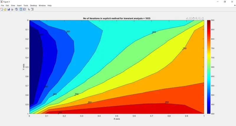
• we set the iterative methos such that it works for error>tolerance.we define the necessary condition such that this loopcan terminate.we set the equation 3 in the loop inorder to get the values of temperature according to explicit method by applying the formula.
• we plot the contour and keep the count of iterations.along with setting of title and label etc.

THE PLOT FOR EXPLICIT METHOD IS AS FOLLOWS:

Now we come to the implicit method whith three iteration method.We use the equation 4 ,prime purpose for solving this problem.

this.

Code for jacobi method

%Transient analysis  jacobi
close all
clear all
clc

%initial parameters
nx=10;
ny=nx;
nt=1400;
x=linspace(0,1,nx);
y=linspace(0,1,ny);

dx=x(2)-x(1);
dy=dx;
error= 9e9;
tolerance=1e-4;
dt=1e-3;

%setting up temeperature conditions
Temperature_Left=400;
Temperature_Top=600;
Temperature_Right=800;
Temperature_Bottom=900;

T=300*ones(nx,ny);


T(2:ny-1,1)=Temperature_Left;
T(2:ny-1,nx)=Temperature_Right;
T(1,2:nx-1)=Temperature_Top;
T(ny,2:nx-1)=Temperature_Bottom;


T(1,1) = (Temperature_Top+Temperature_Left)/2;
T(nx,ny) = (Temperature_Right+Temperature_Bottom)/2;
T(1,ny)=(Temperature_Top+Temperature_Right)/2;
T(nx,1)=(Temperature_Left+Temperature_Bottom)/2;


T_old = T;
T_initial = T;



alpha = 1.4;
k1=alpha*(dt/(dx^2));
k2=alpha*(dt/(dy^2));

jacobi_iteration=1;

for k=1:nt
    error=9e9;
     while(error>tolerance)   %convergence loop
        for i=2:nx-1
            for j=2:ny-1
             Term1=1/(1+(2*k1)+(2*k2));
             Term2=k1*Term1;
             Term3=k2*Term1;
             H=T_old(i-1,j)+T_old(i+1,j);
             V=T_old(i,j+1)+T_old(i,j-1);
             T(i,j)=T_initial(i,j)*Term1+H*Term2+V*Term3;
            end
        end
        
             
       
        error = max(max(abs(T_old - T)));
        T_old = T;
        jacobi_iteration = jacobi_iteration + 1;
     end
     T_initial=T;
end
%plotting
 figure(1)
contour(x,y,T)
clabel(contourf(x,y,T))
colorbar
colormap
colormap(jet)
set(gca,'ydir','reverse')
xlabel('X-axis');
ylabel('Y-axis');
title(sprintf('No of iterations in jacobi method  for transient analysis= %d',jacobi_iteration));
pause(0.0000000003);

Algo for code:

• we define the initial parameters the total number of grid points in x and y axis.
• then we define the uniform distribution of grid points dx and dy.
• we would set the error as 9e9 and tolerance as 1e-4.along with dt .
• As per the question we would define the Temeperature necessary as per question.
• we set the iterative methos such that it works for error>tolerance.we define the necessary condition such that this loopcan terminate.we set the equation 4 in the loop inorder to get the values of temperature according to jacobi method.
• we plot the contour and keep the count of iterations.along with setting of title and label etc.

Plot for implicit jacobi transiet analysis.

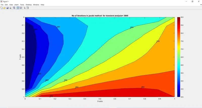
The plot seems to be of wide ranging varying with diffferent values of dx.

The code for Gauss sidel iteration method implicit transient

%Transient analysis  gauss sidel implicit
close all
clear all
clc

%initial parameters

nx=10;
ny=nx;
nt=1400;
x=linspace(0,1,nx);
y=linspace(0,1,ny);

dx=x(2)-x(1);
dy=dx;
error= 9e9;
tolerance=1e-4;
dt=1e-3;


%setting temperature
Temperature_Left=400;
Temperature_Top=600;
Temperature_Right=800;
Temperature_Bottom=900;

T=300*ones(nx,ny);


T(2:ny-1,1)=Temperature_Left;
T(2:ny-1,nx)=Temperature_Right;
T(1,2:nx-1)=Temperature_Top;
T(ny,2:nx-1)=Temperature_Bottom;


T(1,1) = (Temperature_Top+Temperature_Left)/2;
T(nx,ny) = (Temperature_Right+Temperature_Bottom)/2;
T(1,ny)=(Temperature_Top+Temperature_Right)/2;
T(nx,1)=(Temperature_Left+Temperature_Bottom)/2;


T_old = T;
T_initial = T;



alpha=1.4;
k1=alpha*(dt/(dx^2));
k2=alpha*(dt/(dy^2));

gauss_iteration=1;

for k=1:nt
    error=9e9;
     while(error>tolerance)   %converging loop
        for i=2:nx-1
            for j=2:ny-1
             Term_1=1/(1+(2*k1)+(2*k2));
             Term_2=k1*Term_1;
             Term_3=k2*Term_1;
             H=T(i-1,j)+T_old(i+1,j);
             V=T(i,j+1)+T_old(i,j-1);
             T(i,j)=T_initial(i,j)*Term_1+H*Term_2+V*Term_3;
            end
        end
        
             
       
        error = max(max(abs(T_old - T)));
        T_old = T;
        gauss_iteration = gauss_iteration + 1;
     end
     T_initial=T;
end
 figure(1)
contour(x,y,T)
clabel(contourf(x,y,T))
colorbar
colormap
colormap(jet)
set(gca,'ydir','reverse')
xlabel('X-axis');
ylabel('Y-axis');
title(sprintf('No of iterations in gauss sidel method = %d',gauss_iteration));
pause(0.0000000003);

Algo for code:

• we define the initial parameters the total number of grid points in x and y axis.
• then we define the uniform distribution of grid points dx and dy.
• we would set the error as 9e9 and tolerance as 1e-4.along with dt .
• As per the question we would define the Temeperature necessary as per question.
• we set the iterative methos such that it works for error>tolerance.we define the necessary condition such that this loop can terminate.we set the equation 4 in the loop inorder to get the values of temperature according to gauss sidel method.
• we plot the contour and keep the count of iterations.along with setting of title and label etc.

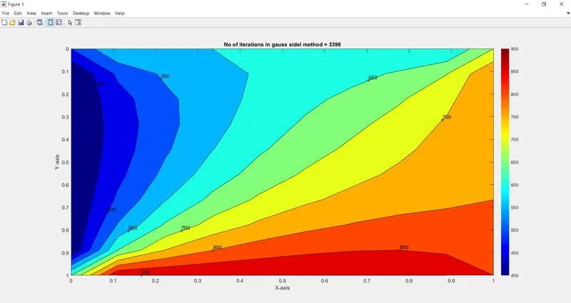
PLOT FOR GAUSS SIDEL METHOD

THE CODE FOR SOR_METHOD

% Transient analysis SOR


close all
clear all
clc

%initial parameters
nx=11;
ny=nx;
nt=1400;
x=linspace(0,1,nx);
y=linspace(0,1,ny);

dx=x(2)-x(1);
dy=dx;
error= 9e9;
tolerance=1e-4;
dt=1e-3;
omega = 1.1;

%setting up the temperature conditions
Temperature_Left=400;
Temperature_Top=600;
Temperature_Right=800;
Temperature_Bottom=900;

T=300*ones(nx,ny);


T(2:ny-1,1)=Temperature_Left;
T(2:ny-1,nx)=Temperature_Right;
T(1,2:nx-1)=Temperature_Top;
T(ny,2:nx-1)=Temperature_Bottom;


T(1,1) = (Temperature_Top+Temperature_Left)/2;
T(nx,ny) = (Temperature_Right+Temperature_Bottom)/2;
T(1,ny)=(Temperature_Top+Temperature_Right)/2;
T(nx,1)=(Temperature_Left+Temperature_Bottom)/2;


T_old = T;
T_initial = T;
T_end=T;



alpha=1.4;
k1=alpha*(dt/(dx^2));
k2=alpha*(dt/(dy^2));

SOR_iteration=1;

for k=1:nt
    error=9e9;
     while(error>tolerance) %convergence loop
        for i=2:nx-1
            for j=2:ny-1
             Term_1=1/(1+(2*k1)+(2*k2));
             Term_2=k1*Term_1;
             Term_3=k2*Term_1;
             H=T(i-1,j)+T_old(i+1,j);
             V=T(i,j+1)+T_old(i,j-1);
             T(i,j)=T_initial(i,j)*Term_1+H*Term_2+V*Term_3;
             T_end(i,j)=((1-omega)*T_old(i,j)+(T(i,j)*omega));
            end
        end
        
             
       
        error = max(max(abs(T_old - T)));
        T_old = T_end;
        SOR_iteration = SOR_iteration + 1;
     end
     T_initial=T_end;
end
%plotting
 figure(1)
contour(x,y,T)
clabel(contourf(x,y,T))
colorbar
colormap
colormap(jet)
set(gca,'ydir','reverse')
xlabel('X-axis');
ylabel('Y-axis');
title(sprintf('No of iterations in SOR  method for transient analysis = %d',SOR_iteration));
pause(0.0000000003);

Algo for code:

• we define the initial parameters the total number of grid points in x and y axis.
• then we define the uniform distribution of grid points dx and dy.
• we would set the error as 9e9 and tolerance as 1e-4.along with dt .
• As per the question we would define the Temeperature necessary as per question.
• we set the iterative methos such that it works for error>tolerance.we define the necessary condition such that this loop can terminate.we set the equation 4 in the loop inorder to get the values of temperature according to SOR method.
• we plot the contour and keep the count of iterations.along with setting of title and label etc.

PLOT FOR SOR_METHOD transient analysis implicit

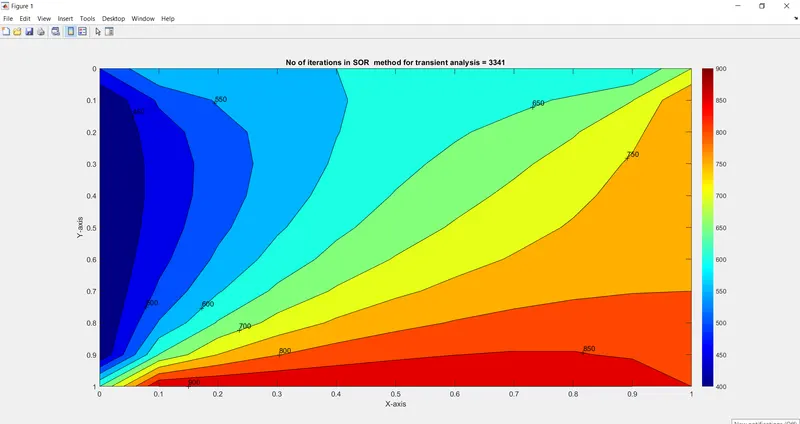
From the plot we could observe the wide range of values for y axis along x -axis.

Now analysis for iteration along implicit and explicit methods.

CONCLUSION:

• Different methods show different no of iterations either it may explicit or implicit or may be its steady or transient.
• In implicit case the no of iterations in Jacobi>Gauss sidel >SOR.
• Explcit method shows a considerable amount of iterations.
• So from these we could say SOR method is best for solving the Implcit equations.