Week 3 - Taylor table method and Matlab code
EXPLANATION OF THE CODE
We start the code with the refreshing statements like clear all, close all, clc.
The schemes used inorder to solve the problem.
1.Skewed Left Difference scheme.
2.Skewed Right Difference scheme.
3.Central Difference scheme.
We define the initial parameters that is
`x =pi/3`
and `dx =`linspace(pi/4,pi/4000,20)
indicates interval with 20 divisions.Then we define the analytical derivative variable with the true value of the function.
We define the for loop inside which we define the variables necessary to be used in different schemes and its value will be stored in array form for various range of values of dx.
Derivation of Expression for various schemes
1.LEFT DIFFERENCE SCHEME
| `f(i)` | `f'(i)*Deltax` | `f''(i)*Deltax^2` | `f'''(i)*Deltax^3` | `f''''(i)*Deltax^4` | `f'''''(i)*Deltax^5` | `f^(vi)(i)*Deltax^6` | |
| `a*f(i)` | a | 0 | 0 | 0 | 0 | 0 | 0 |
| `b*f(i-1)` | b | -b | b/2 | -b/6 | b/24 | -b/120 | b/720 |
| `c*f(i-2)` | c | -2c | 4c/2 | -8c/6 | 16c/24 | -32c/120 | 64c/720 |
| `d*f(i-3)` | d | -3d | 9d/2 | -27d/6 | 81d/24 | -243d/120 | 729d/720 |
| `e*f(i-4)` | e | -4e | 16e/2 | -64e/6 | 256e/24 | -1024e/120 | 4096e/720 |
| `g*f(i-5)` | g | -5g | 25g/2 | -125g/6 | 625g/24 | -3125g/120 | 15625g/720 |
|
sum of coefficients |
0 | 0 | 1 | 0 | 0 | 0 | ? |
a+b+c+d+e+g=0 -(1)
-b-2c-3d-4e-5g=0 -(2)
b/2+4c/2+9d/2+16e/2+25g/2=1 -(3)
-b/6 -8c/6 -27d/6-64e/6-125g/6=0 -(4)
b/24+16c/24+81d/24+81d/24+256e/24+625g/24=0 -(5)
-b/120-32c/120-243d/120-1024e/120-3125g/120 = 0 -(6)
By solving these equations we get all the values.
Derivation of Expression for Left difference scheme.
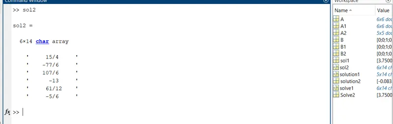
The value of a ,b ,c,d,e,g is calculated from the above relation . The code for solving these values in matrix form is given below the main code.
a= 15/4 , b=-77/6 , c= 107/6 ,d =-13 , e =61/12, g= -5/6
By substituting the above value we can find the sum of coefficients for 6th order we get -0.7611 respectively . -(I)
Hence
Now suppose
`(del^2f)/(delx^2) = (a*f(i)+ b*f(i-1)+c*f(i-2)+ d*f(i-3)+e*f(i-4)+g*f(i-5))/(Deltax^2)` -(1)
By using Taylors expansion we know.
`(del^2f)/(delx^2) = f''(x)*dx^2 *(1)-0.7611*f^(vi)(x)*dx^6`
(where 1 and -0.7611 are the coefficients of 1st and 6th order we deduced that 5th order coefficient sum turns out to be 0).
`(a*f(i)+ b*f(i-1)+c*f(i-2)+ d*f(i-3)+e*f(i-4)+g*f(i-5)) =f''(x)*dx^2 *(1)-0.7611*f^(vi)(x)*dx^6` -(by I)
`(a*f(i)+ b*f(i-1)+c*f(i-2)+ d*f(i-3)+e*f(i-4)+g*f(i-5))/dx^2=f''(x)*(1)-0.7611*f^(vi)(x)*dx^4` (by dividing `dx^2` on both sides.)
`(a*f(i)+ b*f(i-1)+c*f(i-2)+ d*f(i-3)+e*f(i-4)+g*f(i-5))/dx^2 =f''(x)*dx^2 *(1)+O(Deltax^4)`
This expression shows that this is fourth order accurate.
The given situation is of the 4th order accuracy because terms of the order 5 or more are being neglected .Each coloumn in a table has 5 or 6 unknowns.We solve th relation and find the values as above.
2.CENTRAL DIFFERENCE SCHEME
| `f(i)` | `f'(i)*Deltax` | `f''(i)*Deltax^2` | `f'''(i)*Deltax^3` | `f''''(i)*Delta^4` | `f'''''(i)*Deltax^5` | `f^(vi)(x)*Deltax^6` | |
| `a*f(i-2)` | a | -2a | 4a/2 | -8a/6 | 16a/24 | -32a/120 | 64a/720 |
| `b*f(i-1)` | b | -b | b/2 | -b/6 | b/24 | -b/120 | b/720 |
| `c*f(i)` | c | 0 | 0 | 0 | 0 | 0 | 0 |
| `d*f(i+1)` | d | d | d/2 | d/6 | d/24 | d/120 | d/720 |
| `e*f(i+2)` | e | 2e | 4e/2 | 8e/6 | 16e/24 | 32e/120 | 64e/720 |
|
sum of coefficients |
0 | 0 | 1 | 0 | 0 | ? | ? |
a+b+c+d+e=0 -(1)
-2a -b+d+2e=0 -(2)
4a/2+b/2+d/2+4e/2 = 1 -(3)
-8a/6-b/6+d/6+8e/6=0 -(4)
16a/24+b/24+d/24+16e/24 = 0 -(5)
solving these equations we get all the values.
Derivation of Expression for Central difference scheme.
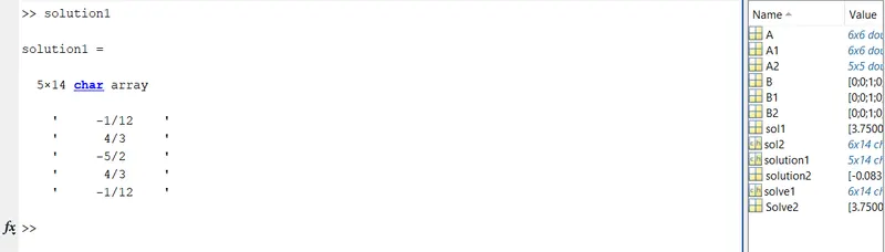
The value of a,b,c,d,e can be calculated from the above relation . The code for solving these values in matrix form is given below the main code.
a=-1/12 ,b= 4/3,c= -5/2, d = 4/3,e = -1/12;
Now suppose
`(del^2f)/(delx^2) = (a*f(i-2)* +b*f(i-1)+c*f(i)+d*f(i+1)+e*f(i+2))/(Deltax^2)`
By substituting the above value we can find the sum of coefficients for 5th and 6th order we get 0 and -0.0111 respectively . -(II)
Hence
By using Taylors expansion we know.
`(del^2f)/(delx^2) = f''(x)*dx^2 *(1)-0.0111*f^(vi)(x)*dx^6`
(where 1 and -0.0111 are the coefficients of 1st and 6th order we deduced that 5th order coefficient sum turns out to be 0 these values are calculated from the table above.).
`(a*f(i-2)* +b*f(i-1)+c*f(i)+d*f(i+1)+e*f(i+2)) =f''(x)*dx^2 *(1)-0.0111*f^(vi)(x)*dx^6` -(by I)
`(a*f(i-2)* +b*f(i-1)+c*f(i)+d*f(i+1)+e*f(i+2))/dx^2=f''(x)*(1)-0.0111*f^(vi)(x)*dx^4` (by dividing `dx^2` on both sides.)
`(a*f(i-2)* +b*f(i-1)+c*f(i)+d*f(i+1)+e*f(i+2))/dx^2=f''(x)*dx^2 *(1)+O(Deltax^4)`
This expression shows that this is fourth order accurate.
The given situation is of the 4th order accuracy because terms of the order 5 or more are being neglected .Each coloumn in a table has 5 or 6 unknowns.We solve th relation and find the values as above.
3.RIGHT DIFFERENCE SCHEME
| `f(i)` | `f'(i)*Deltax` | `f''(i)*Deltax^2` | `f'''(i)*Deltax^3` | `f''''(i)*Deltax^4` | `f'''''(i)*Deltax^5` | `f^(vi)(i)*Deltax^6` | |
| `a*f(i)` | a | 0 | 0 | 0 | 0 | 0 | 0 |
| `b*f(i+1)` | b | b | b/2 | b/6 | b/24 | b/120 | b/720 |
| `c*f(i+2)` | c | 2c | 4c/2 | 8c/6 | 16c/24 | 32c/120 | 64c/720 |
| `d*f(i+3)` | d | 3d | 9d/2 | 27d/6 | 81d/24 | 243d/120 | 729d/720 |
| `e*f(i+4)` | e | 4e | 16e/2 | 64e/6 | 256e/24 | 1024e/120 | 4096e/720 |
| `g*f(i+5)` | g | 5g | 25g/2 | 125g/6 | 625g/24 | 3125g/120 | 15625g/720 |
|
sum of coefficients |
0 | 0 | 1 | 0 | 0 |
0 |
? |
a+b+c+d+e+g=0 -(1)
b+2c+3d+4e+5g=0 -(2)
b/2+4c/2+9d/2+16e/2+25g/2=1 -(3)
b/6 +8c/6 +27d/6+64e/6+125g/6=0 -(4)
b/24+16c/24+81d/24+81d/24+256e/24+625g/24=0 -(5)
b/120+32c/120+243d/120+1024e/120+3125g/120 = 0 -(6)
solving all the equations we cal get all the values
Derivation of Expression for Right difference scheme.
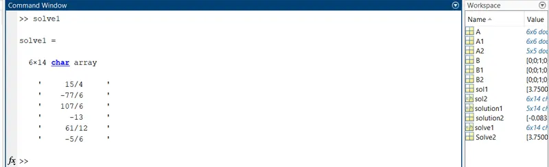
The value of a ,b,c,d,e,g can be calculated . The code for solving these values in matrix form is given below the main code.
a= 15/4, b= -77/6 ,c =107/6,d=-13,e =61/12,g= -5/6
By substituting the above value we can find the sum of coefficients for 5th and 6th order we get 0 and -0.7611 respectively . -(I)
Hence
Now suppose
`(del^2f)/(delx^2) = (a*f(i)+b*f(i+1)+c*f(i+2)+d*f(i+3)+e*f(i+4)+g*f(i+5))/(Deltax^2)` -(1)
By using Taylors expansion we know.
`(del^2f)/(delx^2) = f''(x)*dx^2 *(1)-0.0111*f^(vi)(x)*dx^6`
(where 1 and -0.7611 are the coefficients of 1st and 6th order we deduced that 5th order coefficient sum turns out to be 0).
`(a*f(i)+b*f(i+1)+c*f(i+2)+d*f(i+3)+e*f(i+4)+g*f(i+5)) =f''(x)*dx^2 *(1)-0.7611*f^(vi)(x)*dx^6` -(by I)
`(a*f(i)+b*f(i+1)+c*f(i+2)+d*f(i+3)+e*f(i+4)+g*f(i+5))/dx^2=f''(x)*(1)-0.7611*f^(vi)(x)*dx^4` (by dividing `dx^2` on both sides.)
`(a*f(i)+b*f(i+1)+c*f(i+2)+d*f(i+3)+e*f(i+4)+g*f(i+5))/dx^2 =f''(x)*dx^2 *(1)+O(Deltax^4)`
This expression shows that this is fourth order accurate.
The given situation is of the 4th order accuracy because terms of the order 5 or more are being neglected .Each coloumn in a table has 5 or 6 unknowns.We solve th relation and find the values as above.
From these they could be substituted in the equation
`(del^2f)/(delx^2) = (a*f(i)+ b*f(i-1)+c*f(i-2)+ d*f(i-3)+e*f(i-4)+g*f(i-5))/(Deltax^2)` --This is for the left difference scheme`
`(del^2f)/(delx) = (a*f(i)+b*f(i+1)+c*f(i+2)+d*f(i+3)+e*f(i+4)+g*f(i+5))/(Deltax^2)`--This is for the
right difference scheme
`(del^2f)/(delx^2) = (a*f(i-2)* +b*f(i-1)+c*f(i)+d*f(i+1)+e*f(i+2))/(Deltax^2)`
This is for the central difference scheme
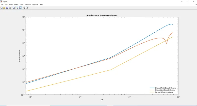
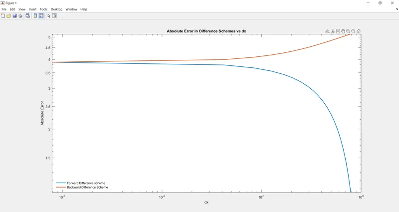
Then we plot all the equaitons we have derived in the reasonable manner.with the log scale.with appropriate legend and title.The two plots will be plotted respectively.
Conclusion from the plot ,it seems that the central difference error is smalller comapred to the skewed rigth and skewed left difference scheme.
The central difference starts from somewhere around `10^-9` and increases drastically.This is similar in the case of Skewed right and Skewed left difference scheme.
Derivation for the schemes to be fourth order accurate
THE CODE FOR THE ABOVE EXPLANATION
clear all
 close  all
 clc

 %initial parameters

 x= pi/3;
 dx =linspace(pi/4,pi/4000,20);

 analytical_derivative = -2*exp(x)*sin(x);

 for i = 1:length(dx)


     al(i) = (exp(x- 5*dx(i)))*(cos(x-5*dx(i)));
     bl(i) = (exp(x- 4*dx(i)))*(cos(x- 4*dx(i)));
     cl(i) = (exp(x - 3*dx(i)))*(cos(x -3*dx(i)));
     dl(i) = (exp(x - 2*dx(i)))*(cos(x -2*dx(i)));
     el(i) = (exp(x - 1*dx(i)))*(cos(x -1*dx(i)));
     f(i)=(exp(x))*(cos(x));
     ar(i) = (exp(x + 1*dx(i)))*(cos(x +1*dx(i)));
     br(i) =(exp(x + 2*dx(i)))*(cos(x +2*dx(i)));
     cr(i) = (exp(x +3*dx(i)))*(cos(x +3*dx(i)));
     dr(i) = (exp(x +4*dx(i)))*(cos(x +4*dx(i)));
     hr(i) = (exp(x +5*dx(i)))*(cos(x +5*dx(i)));

     fds(i) = (ar(i) - f(i))/(dx(i));
     bds(i) = (f(i) -el(i))/(dx(i));
     cds(i) = (-dl(i)+16*el(i) -30*f(i) +16*ar(i)-br(i))/(12*dx(i)^2);

     skew_left(i) = (45*f(i) -154*el(i) +214*dl(i) -156*cl(i) +61*bl(i)-10*al(i))/(12*dx(i)^2);
     skew_right(i) = (45*f(i) -154*ar(i) +214*br(i) -156*cr(i) +61*dr(i)-10*hr(i))/(12*dx(i)^2)

     error_forward(i) = abs(fds(i) - analytical_derivative);
     error_backward(i) = abs(bds(i) - analytical_derivative);
     error_central(i) = abs(cds(i) - analytical_derivative);
     error_left(i) = abs(skew_left(i) - analytical_derivative);
     error_right(i) =abs(skew_right(i) - analytical_derivative);

 end


 figure(1)
 loglog(dx,error_forward,'linewidth',1.5);
 xlabel('dx');
 ylabel('Absolute error');
 title('Absolute Error in Difference Schemes vs dx');

 hold on
 loglog(dx,error_backward,'linewidth',1.5);
 xlabel('dx');
 ylabel('Absolute Error');
 legend('Forward Difference scheme','Backward Difference Scheme','Location','southwest');
figure(2)
 loglog(dx,error_right,'linewidth',1.5);
 xlabel('dx');
 ylabel('Absolute Error');
 title('Absolute error in various schemes');

 hold on
  loglog(dx,error_left,'linewidth',1.5);
  xlabel('dx');
  ylabel('Absolute error');

  hold on
   loglog(dx,error_central,'linewidth',1.5);
   xlabel('dx');
   ylabel('Absolute error');

legend('Skewed Right Sided Difference','Skewed Left Sided Difference','Central Difference scheme','Location' ,'southeast');
THE CODE FOR SOLVING THE VALUES OF a,b,c,d,e,g
%left   difference  scheme
A=[ 1 1 1 1 1 1;0 -1 -2 -3 -4 -5; 0 1/2 4/2 9/2 16/2 25/2 ; 0 -1/6 -8/6 -27/6 -64/6 -125/6;0 1/24 16/24 81/24 256/24 625/24 ;0 -1/120 -32/120 -243/120 -1024/120 -3125/120];
B= [ 0 ; 0 ; 1 ; 0 ; 0 ; 0 ];

sol2=rats(linsolve(A,B));
sol1= inv(A)* B


%right difference scehme
A1 = [ 1 1 1 1 1 1;0  1  2  3  4  5; 0 1/2 4/2 9/2 16/2 25/2 ; 0  1/6  8/6  27/6  64/6  125/6;0 1/24 16/24 81/24 256/24 625/24 ;0  1/120  32/120  243/120  1024/120  3125/120];
B1= [ 0 ; 0 ; 1 ; 0 ; 0 ; 0 ];

solve1=rats(linsolve(A1,B1));
Solve2=inv(A1)* B1

%central differnece scheme
A2=[ 1 1 1 1 1 ;-2 -1 0 1 2 ;4/2 1/2 0 1/2 4/2;-8/6 -1/6 0 1/6 8/6;16/24 1/24 0 1/24 16/24];
B2=[0 ;0;1;0;0];
solution1=rats(linsolve(A2,B2));
solution2=inv(A2)*B2;
This code shows the output for the solution of linear systems.
THE OUTPUT FOR THE LINEAR SYSTEMS
THE OUTPUT FOR THE LEFT DIFFERENCE SCHEME
THE OUTPUT FOR THE RIGHT DIFFERENCE SCHEME
THE OUTPUT FOR THE CENTRAL DIFFERENCE SCHEME
THE OUTPUT PLOTS
Why a skewed scheme is useful ? what can a skewed scheme do that a CD scheme cannot do?
- The skewed scheme works well when we need to calculate all the points one side in more systematic manner ,for calculating node on one side with higher approximation we need the skewed scheme as comaritively to the central difference scheme .we could take an example of oil flowing from heigth to down wards .The behaviour of the upstream side can be uswed to calculate the flow in downstream.However the central difference scheme cannot be used to calculate the corner nodes with higher approximations.In central difference scheme depends on both sides ,not every time information regarding the flow is available in both sides in case of CDS.
- By comapring the plots we come to the conclusion reagrding the error that CDS scheme contains less error comparitively.Thats why it is preffered that using CDS to solve equations will provide accurate results with fewer errors.
.
From the above the comparision of different schemes for fourth order approximation of a second order derivative ,we can reassure that the central difference scheme approximation yields more accurate solutions than the right -skewed and left -skewed differencing schemes .since forward and backward approximations are of second order error they give out large errors than the other fourth order schemes.
It may also be noted that if we consider a wider range of dx ,at some values of dx the error produced by higher order schemes is bigger than that of lower order schemes .This is due to higher roundoff errors at these points.It is important to understand that the value of error at any point is the net sum of numerical erro and round off error.And this truncation error increases with increase in order.Therefore higher order schemes may not be a good option to choose.