Week 9 - FVM Literature Review

Finite difference method	Finite volume method
Easy to implement	Complicated then finite difference method
The dependent variables are stored at nodes only	The dependent variables are stored in center of finite volume
The discretization is based on partial differential equations	The discretization is based on integral form of partial differential equations
Differential scheme brings some approximation error	Integral scheme, since we are integrating across area chance of error is minimized.
Differential schemes are faster	Integral schemes are slightly slower but score over finite difference scheme
This method uses a topologically square network of lines to construct the discretization which makes it restricted towards solving complex geometries	The shapes used in finite volume method can be any since we are considering control volume

The approximation of surface and volume integrals require values of the variable at locations other than the computational nodes of the control volume, the values at this nodes are obtained using interpolation schemes.

Interpolation schemes:

• Upwind interpolation
• Linear interpolation
• Quadratic upwind interpolation
• Hybrid interpolation
• Total variation diminishing schemes

The commonly used schemes are upwind, linear, and quadratic interpolation.

Upwind interpolation schemes:

The name itself define it, the upwind in term the values are calculated at upstream nodes.

The upwind interpolation scheme for approximating the value of the variable ‘f’ at the east face of the control volume is given as.

f_e = f_p if (v.n)_e > 0

f_e if (v.n)_e < 0

This is equivalent to backward and forward finite difference approximation, it is first order accurate.

Advantage:

• The solution is always bounded

Dis-advantages:

• It is numerically diffusive in nature.
• Peaks or rapid variations in the variables are smeared out.

Linear interpolation schemes/central difference scheme:

In this method the value of variables are approximated at the face centre of control volume for two nearest computational nodes.

f_e = f_e λ_e + f_p (1 - λ_e )

where,

λ_e = (X_e - X_p) / (X_E – X_P)

It is equivalent to the use of central difference formula of the first order derivative.

Advantages:

• It is most widely used interpolation scheme leads to a very simple approximation for evaluation of gradients required for evaluation of diffusive fluxes.
• Approximation of gradients has a second order accuracy on uniform grids.

Dis-advantages:

• This scheme may produce oscillatory effects.

Question arises can we get better scheme which has better damping properties then central differencing scheme and better accuracy then upwind differencing scheme.

Quick upwind interpolation:

In this method we approximate the value of the variables at control volume face centre by quadratic interpolation of the values at three nearest computational nodes (1 downstream node and 2 upstream nodes).

f_e = f_u + G₁ (f_d - f_u) + G₂ (f_uu – f_u)

G₁ = (X_e - X_u) (X_e - X_uu) / (X_p – X_u) (X_p – X_uu)

G₁ = (X_e - X_u) (X_e - X_p) / (X_uu– X_u) (X_uu – X_p)

It is third order accurate scheme on both uniform and non-uniform grids.

Hybrid interpolation schemes:

Blend of central differencing and upwind differencing scheme based on peclet number.

f­_e = λ f_CDS - (1 – λ) f_UDS

Total variation diminishing (TVD) scheme:

f­_e = f_d + (1/2)*ψ(r)*(f_E – f_p )

Flux limiter:

Before discussing the flux limiter the terminology with which we should be familiar with is high resolution schemes.

High-resolution schemes are used in the numerical solution of partial differential equation where high accuracy is required in the presence of shocks or discontinuities. They have the following properties:

• Second- or higher-order spatial accuracy is obtained in smooth parts of the solution.
• Solutions are free from spurious oscillations or wiggles.
• High accuracy is obtained around shocks and discontinuities.
• The number of mesh points containing the wave is small compared with a first-order scheme with similar accuracy.

Most of us might have seen the behavior of numerical schemes in order to capture shocks and discontinuity that arises in hyperbolic equations. Physically, these equations model the convective fluid flow. It has been observed that low-order schemes are usually stable but quite dissipative in nature around the points of discontinuity/shocks. On the other hand higher-order numerical schemes are unstable in nature and show oscillations in the vicinity of discontinuity. One can have a better understanding of such behavior by analyzing the modified equation of these schemes.

Now as said above one cannot have high order accuracy without oscillations. The objective is to have highly accurate and stable oscillation free schemes. This kind of schemes are known as high resolution schemes. In 1984 Harten proposed the construction and gave TVD criteria for such scheme. Here we talk only about using flux limiters function to construct high resolution schemes. The idea is to tune the numerical flux of high order and low order scheme using the flux limiter function in such a way that the resulting scheme gives a high order accuracy in the smooth region of flow and sticks with first order of accuracy in the vicinity of socks/discontinuities as follows:

Define the numerical flux function of high resolution conservative scheme as

Where L, H are the numerical flux of conservative low order and high order schemes respectively. And is a function of smoothness parameter usually defined as

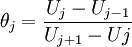
What remains next is to define the limiter function in such a way that it satisfies at least the following properties:

• remains positive ,
• satisfies
• Passes through a particular region known as TVD region associated with the underlying scheme in order to guarantee stability of the scheme.