The Finite Volume Method (FVM)

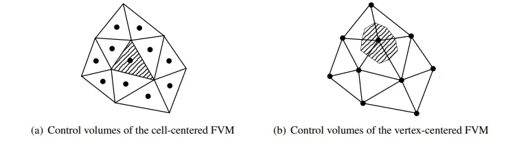
The Finite Volume Method (FVM) is one of the most versatile discretization techniques used in CFD. Based on the control volume formulation of analytical fluid dynamics, the first step in the FVM is to divide the domain into a number of control volumes (aka cells, elements) where the variable of interest is located at the centroid of the control volume. The next step is to integrate the differential form of the governing equations (very similar to the control volume approach) over each control volume. Interpolation profiles are then assumed in order to describe the variation of the concerned variable between cell centroids. The resulting equation is called the discretized or discretization equation. In this manner, the discretization equation expresses the conservation principle for the variable inside the control volume. The most compelling feature of the FVM is that the resulting solution satisfies the conservation of quantities such as mass, momentum, energy, and species. This is exactly satisfied for any control volume as well as for the whole computational domain and for any number of control volumes. Even a coarse grid solution exhibits exact integral balances.

Finite Difference Method (FDM):

Finite Difference Method is most used method for the CFD discretization. In which we calculate the variables at different points at discretize points. the problem domain is discretized so that the values of the unknown dependent variables are considered only at a finite number of nodal points instead of at every point over the domain. sider, as an example, a differential problem to be solved in a one-dimensional spatial domain of length L, which involves only the independent variable x in Cartesian coordinates. In the finite difference method, the domain 0 ≤ x ≤ L is discretized—let us say in equal segments of length Δx, where Δx = L/M, thus generating a grid (or mesh) of (M + 1) nodes in the spatial domain.

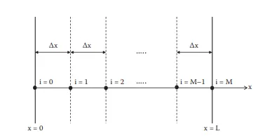
Therefore, (M + 1) algebraic equations are developed by discretizing the governing differential equations and the boundary conditions for the problem. The problem of solving the ordinary or partial differential equations over the problem domain is then transformed to the task of development of a set of algebraic equations and their solution by a suitable algorithm.

1D linear heat conduction equation:

This is 3D transient heat transfer equation with heat generation

Now the 1D steady heat transfer equation with heat generation(source term) is

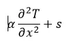
Now the heat transfer profile is divider into the small control volume and 1,2,3,4,5 are center of the volume.

Now consider the control volume 2

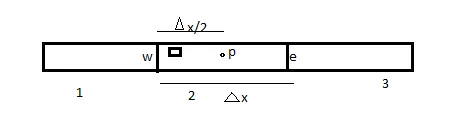
Here 'e' is center point of the east face and w is the center point of the west face and p is the center point of the concentrated volume.

In the control volume 2 there is a small control volume is there. in this control volume the 1D heat conduction equation is conserved so

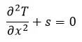
Now integrate for the volume 2

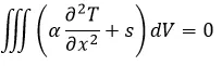
It is a one dimensional heat equation, so the volume dV=A.dx

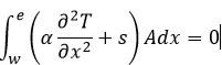
After integration we found

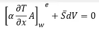
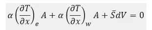
after interpolation

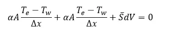
Now

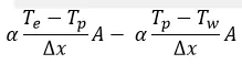term is the flux term this is due to

Interpolation scheme is use to calculate the flux terms in the centrode of the control volume and at the centrode of face.

These are the interpolation scheme:

1. Second order upwind differencing (SOU)

2. linear upwind differencing (LUD)

3. Beam-Warming (BW)

For highly convective flow and where the gradient term is very high or due to any sock formation there is a possible of solution become unbounded.

For that we use the flux limiter, When the limiter detects strong gradients or changes in slope, it switches locally to low resolution (upwind). The concept of the limiter function is based on monitoring the ratio of successive gradients.

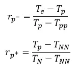
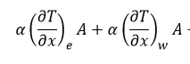term is the gradient flux term.

To find out the gradient of the flux in the face center and in the center of the control volume is use the gradient scheme .

To find the gradient inside the control volume we can use following scheme.

(1) least squares

(2)Gauss, node-based reconstruction

(3)Gauss