Project 2 - Rankine cycle Simulator
AIM - Rankine cycle Simulator
Theory:
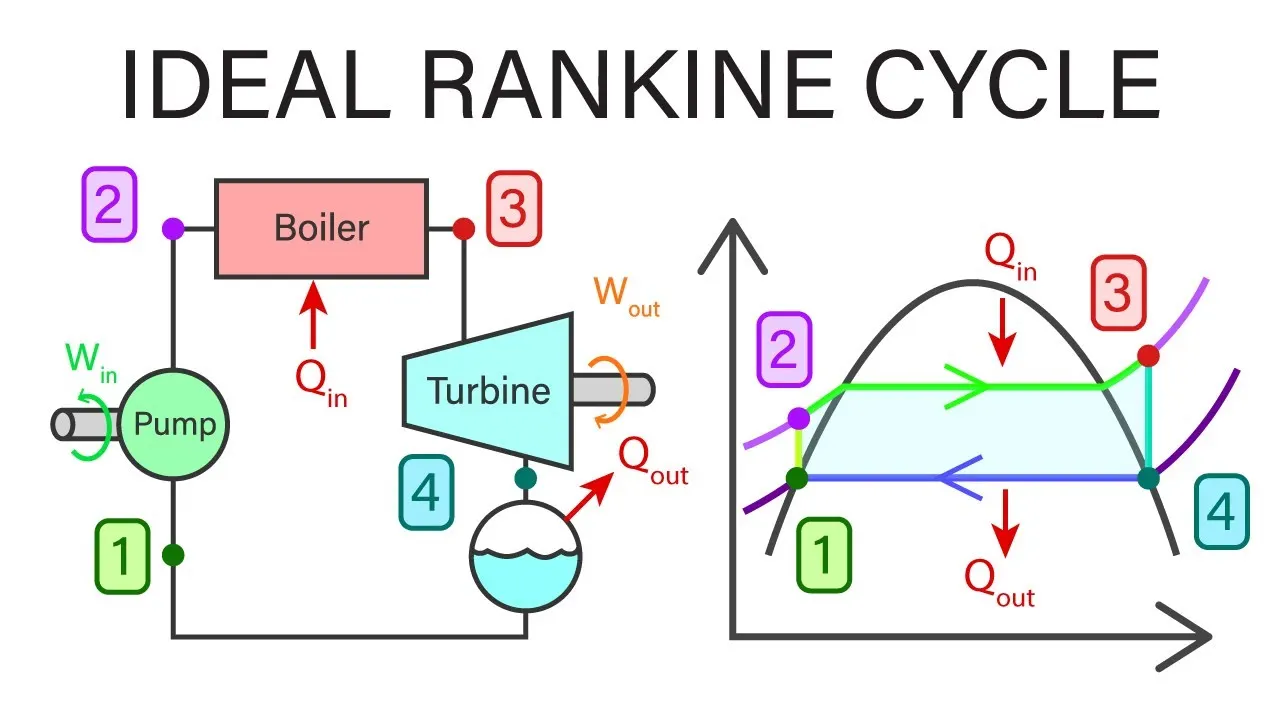
Rankine cycle: The Rankine cycle or Rankine Vapor Cycle is the process widely used by power plant such as coal fired engine or nucular powered engine. In this mechanism, a fuel is used to produce heat within a boiler, converting water into steam which then expands through a turbine producing useful work. This process was developed in 1859 by Scottish engineer William J.M. Rankine. This is a thermodynamic cycle which converts heat into mechanical work—which usually gets transformed into electricity by .
The steps in the Rankine Cycle:
Pump: Compression of the fluid to high pressures using a pump. here fluid was compressed in a isoentropic process.
Boiler: The compressed fluid is heated to the final temperature, here heat was added in a constant pressure process .
Turbine: Expansion of the vapor in the turbine. here we get work output in a isoentropic process .
Condenser: Condensation of the vapor in the condenser, here costand tempreture cooling take place .
'XSteam' function :
clear all
close all
clc

%state 1 inlet of turbine
%pressure in bar
%tempreture in degc
%Enthalpy    (kJ/kg)
%Specific entropy (kJ/kg-K)
%state 1
p1=30
t1=400
h1=XSteam('h_pT',30,400)
s1=XSteam('s_pT',30,400)
%state 2 outlet of turbine
p2=0.05
s2=s1
t2=XSteam('T_ps',0.05,s2)
x=XSteam('x_ps',0.05,s2)
h2=XSteam('h_px',0.05,x)
%state 3
p3=0.05
t3=t2
h3=XSteam('hL_T',t3)
s3=XSteam('sL_T',t3)
%state 4
p4=30
s4=s3
t4=XSteam('T_ps',30,s4)
h4=XSteam('h_pT',30,t4)
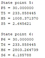
%state 5
p5=30
t5=XSteam('Tsat_p',30)
s5=XSteam('sL_T',t5)
h5=XSteam('hL_T',t5)
%state 6
p6=30
t6=t5
h6=XSteam('hV_p',p5)
s6=XSteam('sV_p',p5)
%calculate the Net work output
%Net work output=Turbine work output(w1)-pump ouput(w2)
w1=h1-h2
w2=h3-h4
w=w1-w2
% Back work ratio
Back_work_ratio = (h4-h3)/(h1-h2);
%creat the tampreture array
T = linspace(0,400,1000);
%plot the saturated line
for i=1:length(T)
    sf(i)=XSteam('sL_T',T(i));
    sg(i)=XSteam('sV_T',T(i));
    hf(i)=XSteam('hL_T',T(i));
    hg(i)=XSteam('hV_T',T(i));
end
%plot of rankine
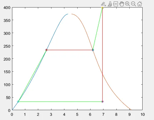
figure(1)
plot(sf,T)
hold on
plot(sg,T)
plot(s1,t1,'*')
plot(s2,t2,'*')
plot(s3,t3,'*')
plot(s4,t4,'*')
plot(s5,t5,'*')
plot(s6,t6,'*')
plot([s1,s2],[t1,t2],'color','r')
plot([s2,s3],[t2,t3],'color','g')
plot([s3,s4],[t3,t4],'color','r')
plot([s4,s5],[t4,t5],'color','g')
plot([s5,s6],[t5,t6],'color','r')
plot([s6,s1],[t6,t1],'color','g')
%plot h-s digram
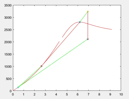
figure(2)
plot(sf,hf,'Color','r')
hold on
plot(sg,hg,'Color','r')
plot(s1,h1,'*')
plot(s2,h2,'*')
plot(s3,h3,'*')
plot(s4,h4,'*')
plot(s5,h5,'*')
plot(s6,h6,'*')
plot([s1,s2],[h1,h2],'color','r')
plot([s2,s3],[h2,h3],'color','g')
plot([s3,s4],[h3,h4],'color','r')
plot([s4,s5],[h4,h5],'color','g')
plot([s5,s6],[h5,h6],'color','r')
plot([s6,s1],[h6,h1],'color','g')
% Displaying Results
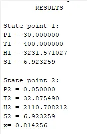
fprintf('        RESULTS\n\n')
fprintf('State point 1:\n')
fprintf('P1 = %f\n',p1)
fprintf('T1 = %f\n',t1)
fprintf('H1 = %f\n',h1)
fprintf('S1 = %f\n\n',s1)

fprintf('State point 2:\n')
fprintf('P2 = %f\n',p2)
fprintf('T2 = %f\n',t2)
fprintf('H2 = %f\n',h2)
fprintf('S2 = %f\n',s2)
fprintf('x= %f\n\n',x)

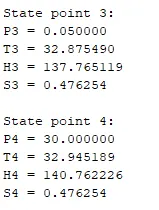
fprintf('State point 3:\n')
fprintf('P3 = %f\n',p3)
fprintf('T3 = %f\n',t3)
fprintf('H3 = %f\n',h3)
fprintf('S3 = %f\n\n',s3)

fprintf('State point 4:\n')
fprintf('P4 = %f\n',p4)
fprintf('T4 = %f\n',t4)
fprintf('H4 = %f\n',h4)
fprintf('S4 = %f\n\n',s4)

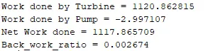
fprintf('Work done by Turbine = %f\n',w1)
fprintf('Work done by Pump = %f\n',w2)
fprintf('Net Work done = %f\n',w)
fprintf('Back_work_ratio = %f\n',Back_work_ratio)
Metlab code explanation :
Turbine Inlet temperature = 400° C
Turbine Inlet Pressure = 30 bars
Turbine Outlet Pressure = 0.05 bars = Condenser Inlet Pressure