Week 5 - Genetic Algorithm

Objective-Genetic Algorithm

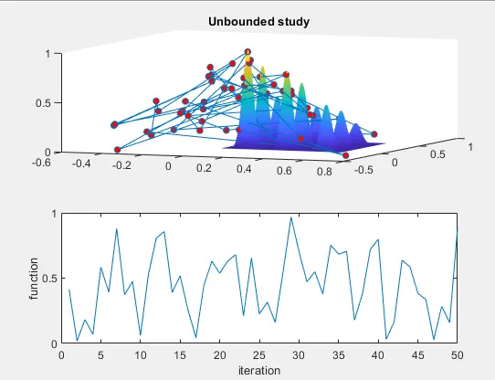
What is GA :- GA is a search based optimization techniques, which is based on genratic and natural selection processes .It is ferquently use on optimal and near optimal solution.

Types of GA study:

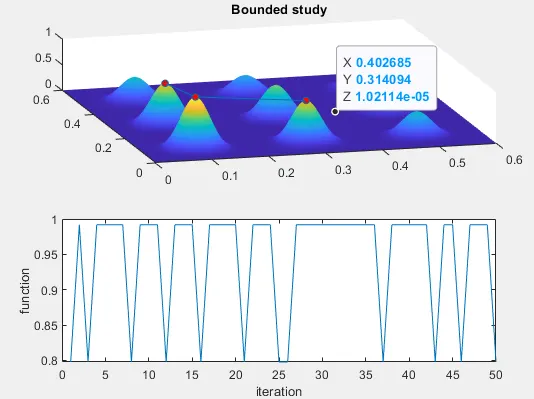
1.bounded study

2.Unbounded study

3.bounded study with population size

syntex:

x=ga(fun,nvars,A,b,Aeq,beq,lb,ub,nonlocn,options)

fun- Objective function

nur-number of veriables

A,b-linear in equality constains

A-real metrix and b=Real vactor

Aeq, Beq- Liner equality constain .

Lb, Ub- Lower and Upper bounds .

non locon-Non linner constain .

Option- Optimization option

options = optimoptions(SolverName,Name,Value)

returns options with specified parameters set using one or more name-value pair arguments

MATLAB CODE:

clear all
close all
clc

%defining our search space
x=linspace(0,0.6,150);
y=linspace(0,0.6,150);
[xx yy]=meshgrid(x,y);

numbercase =50;
%Evaluation the stalagmite function
for i=1:length(xx)
    for j=1:length(yy)
        input_vector(1)=xx(i,j);
        input_vector(2)=yy(i,j);
        f(i,j)=stalamite(input_vector);
    end
end
tic
%unbounded study
for i=1:numbercase
    [m,fval(i)]=ga(@stalamite,2);
    xopt(i)=m(1);
    yopt(i)=m(2);
end
toc
study_time1=toc
 %plot result of study1
 figure(1)
 subplot(2,1,1)
 hold on
 surf(xx,yy,-f)
 shading interp
 plot3(xopt,yopt,-fval,'Marker','o','MarkerSize',5,'markerfacecolor','r')
 title('Unbounded study')
 subplot(2,1,2)
 plot(-fval)
 xlabel('iteration')
 ylabel('function')
 tic
 %bounded study
 for i=1:numbercase
    [m,fval(i)]=ga(@stalamite,2,[],[],[],[],[0;0],[0.6;0.6]);
    xopt(i)=m(1);
    yopt(i)=m(2);
 end
 toc
 figure(2)
 subplot(2,1,1)
 hold on
 surf(xx,yy,-f)
 shading interp
 plot3(xopt,yopt,-fval,'Marker','o','MarkerSize',5,'markerfacecolor','r')
 title('Bounded study')
 subplot(2,1,2)
 plot(-fval)
 xlabel('iteration')
 ylabel('function')
  tic
 %bounded study2
 for i=1:numbercase
    options =optimoptions('ga','PopulationSize',200); % options 'Syntax'
    [m,fval(i)]=ga(@stalagmite,2,[],[],[],[],[0,0],[1,1],[],options); % ga 'syntax'
    xopt(i)=m(1);
    yopt(i)=m(2);
 end
 toc
 figure(3)
 subplot(2,1,1)
 hold on
 surf(xx,yy,-f)
 shading interp
 plot3(xopt,yopt,-fval,'Marker','o','MarkerSize',5,'markerfacecolor','r')
 title('Bounded study')
 subplot(2,1,2)
 plot(-fval)
 xlabel('iteration')
 ylabel('function')

STALGMITE FUNCTION:

function [f]=stalamite(input_vector)
    x=input_vector(1);
    y=input_vector(2);
    term1=(sind(5.1*180*x+0.5))^6;
    term2=(sind(5.1*180*y+0.5))^6;
    term3=exp(-4*log(2)*((x-0.0667)^2/0.64));
    term4=exp(-4*log(2)*((y-0.0667)^2/0.64));
    f=-(term1*term2*term3*term4);
end

CODE EXPLANATION :

'f(i,j)=stalamite(input_vector);' To call the stalamite function .

'f(i,j)=stalamite(input_vector);' To calling the stalamite function .

'tic_toc' Is use to calculate the total time taken to complete to the process .

'[m,fval(i)]=ga(@stalamite,2)' To call the genaratic algorithm in Nonbounded study .

'subplot(2,1,1)' To plot multiple plot in a single figer .

'surf(xx,yy,-f)' To plot the stlgamite function .

'shading interp' To clear the in the shading in the plot .

'plot3'It is use to 3 variable in a Plot .

'[m,fval(i)]=ga(@stalamite,2,[],[],[],[],[0;0],[0.6;0.6]);' To call the genaratic algorithm in Nonbounded study .

'options =optimoptions('ga','PopulationSize',200);'returns options with specified parameters set using one or more name-value pair arguments.

'[m,fval(i)]=ga(@stalagmite,2,[],[],[],[],[0,0],[1,1],[],options)' It is use to call the ga function of unbounded study with population size .

OUTPUT OF MATELAB CODE :

INNCORRECT MATLAB CODE:

figure(1)
 subplot(2,1,1)
 hold on
 surf(xx,yy,f)
 shading interp
 plot3(xopt,yopt,fval,'Marker','o','MarkerSize',5,'markerfacecolor','r')
 title('Unbounded study')
 subplot(2,1,2)
 plot(-fval)
 xlabel('iteration')
 ylabel('function')

function [f]=stalamite(input_vector)
    x=input_vector(1);
    y=input_vector(2);
    term1=(sind(5.1*180*x+0.5))^6;
    term2=(sind(5.1*180*y+0.5))^6;
    term3=exp(-4*log(2)*((x-0.0667)^2/0.64));
    term4=exp(-4*log(2)*((y-0.0667)^2/0.64));
    f=(term1*term2*term3*term4);
end

INCORRECT CODE OUTPUT

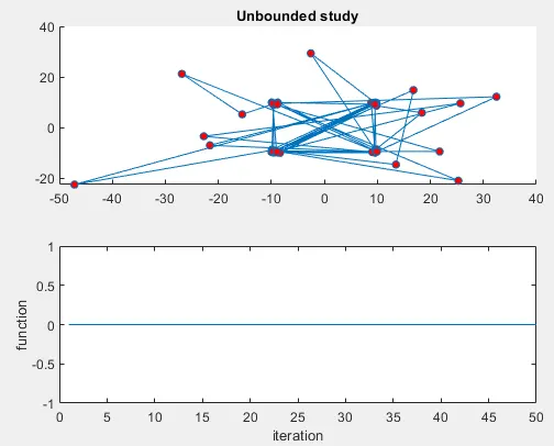
Here output was wrong because stalgmite function was wrong .So correct the function and in plot use '-f' and '-fval' for proper output .

Conclusion :

(1) In bounded study We get less no of minmal value then nonbounded value , so it will be easy to find the minmal value in bounded study.

(2) We will get more aqurate optimum value by useing the bounded study with population size