Week 9 - FVM Literature Review

Finite Volume Method (FVM):

This is one of the discretization methods in which the governing partial differential equations are evaluated inside finite control volumes and are then converted to algebraic equations.

In this, the geomtery is divided into control volumes of any arbitrary shape and the governing equations are evaluated over the entire the control volume.

In Finite Difference Method (FDM), the geometry is divided into structured grids and the governing equations are evaluated at the grid points. But if the geomtery is very complex, it cannot be divided into a structured grid following X, Y and Z directions. FDM calculates properties at a particular point based on the properties of surrounding grid points in X, Y and Z directions. But if the geometry cannot be divided along the cartesian axes, the properties at a particular grid point cannot be evaluated. For this purpose, FVM is used. Here geometry can be of any arbitrary shape and is divided into control volumes. The governing equations are written at the centre point of the control volume and is then integrated along the whole control volume.

For example, let us apply FVM to 1D steady state heat conduction equation.

`d/dx*(k*(dT)/dx) + S= 0` --> (1)

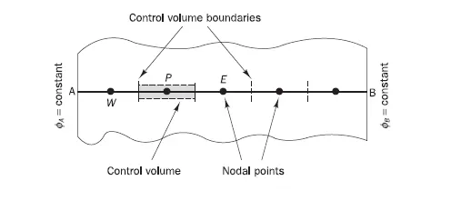
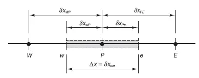
First step is to divide the domain into discrete control volumes and nodal points are placed in between boundaries. The face of the control volume is placed at the middle of two nodes.

The distances between nodes and naming of nodal points is given as

The next step is to integrate the governing equation over the control volume.

`int_(CV) d/dx*(k*(dT)/dx)dV + int_(CV)S dV = 0`

dV = A*dx

Therefore, `(k*A*(dT)/dx)_w^e + S^' dV = 0`

`k_e*A*((dT)/dx)_e - k_w*A*((dT)/dx)_w + S^'dV = 0` --> (2)

The above equation shows us that the heat flux leaving minus the heat flux entering is equal to heat generation. The equation states that the heat flux is balanced. The mathematical form respresents the physical meaning whereas in FDM, the mathematical form obtained after discretizing does not repersent any physical meaning.

The thermal conductivity is a function of temperature. So, they are different for each face w and e.

To obtain the values of T at P, the values of gradients and diffusion coefficient (thermal conductivity) must be known.

These can be approximated using various interpolation schemes.

1. Central Differencing scheme:

In this, the flux gradients are evaluated by considering the flux values of the adjacent nodes.

In the above case, the temperature gradient at east face and west face can be wriiten as

`k_e*A*((dT)/dx)_e = k_e*A*(T_E - T_P)/dx`

`k_w*A*((dT)/dx)_w = k_w*A*(T_P-T_W)/dx`

The source term is a function of dependent variable and can be written as `S^' = S_u + S_P*phi_P`

Therefore equation (2) becomes

`k_e*A*(T_E - T_P)/dx - k_w*A*(T_P - T_W)/dx + (S_u + S_P*T_P)= 0`

Accuracy of the scheme is of second order. This scheme is suitable to use for diffusion problems. But when it is used for convection diffusion problems, this scheme has some limitations. When the peclet number at any one of the faces is greater than 2, the solution becomes unstable. This is because the convective term dominates the diffusive term. Also this scheme does not have the transportiveness property. This scheme considers the values of the adjacent nodes only even when the convective term dominates. Adjacent node values must be taken only during diffusion because the information flow is from all sides. But during convection, the information flow is only from a particular direction i.e., properties at a particular point are influenced only from one direction.

2. Upwind differencing scheme:

To overcome the above problem of central differencing scheme in not being able to identify the flow of information, this scheme is used in which the flow direction is taken into account for determing values at cell faces.

So, in a convection diffusion problem, if the flow is from west to east,

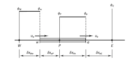
temperature at west face, `T_w = T_W`

temperature at east face, `T_e = T_P`

If the flow is from east to west,

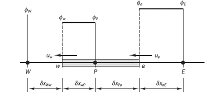
temperature at west face, `T_w = T_P`

temperature at east face, `T_e = T_E`

In this way, the transportiveness property is satisfied. Also, the solution obtained will be stable. But the accuracy of the scheme is of first order. Therefore, it cannot produce accurate results.

3. Hybrid differencing scheme:

This scheme is a combination of central and upwind differencing schemes. For peclet numbers less than 2, central differencng scheme is used and for higher than 2, upwind scheme is used. This scheme uses piecewise formulae on local peclet number to evaluate flux values at each face. Therefore, it satisfies the transportiveness property by using central differencing scheme when diffusion is dominant and uses upwind scheme when convection is dominant.

But the accuracy of this scheme is still of first order for highly convective flows.

4. Quadratic Upstream Interpolation for Convective Kinetics (QUICK):

The scheme that gives stable solution are of first order accuracy. This reduced the accuracy due to artificial viscosity. Therefore, higher order accurate schemes should be used. The QUICK scheme is of third order accuracy. It uses a three point upstream weighted quadratic interpolation for cell face values. A quadratic function is used to obtain flux values at faces.

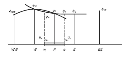
For a uniform grid, the value of `phi`at the cell face between two bracketing nodes i and i-1 and upstream node i-2 is given by

`phi_(face) = 6/8*phi_(i-1) +3/8*phi_(i) -1/8*phi_(i-2)`

temperature at west face will be

`T_(w) = 6/8*T_(W) +3/8*T_(P) -1/8*T_(WW)`

temperature at east face will be

`T_(e) = 6/8*T_(P) +3/8*T_(E) -1/8*T_(W)`

This scheme satisfies the transportiveness property as it considers two upstream and one downstream values.

But this scheme gives rise to stabilty problems under certain flow conditions. This can be solved by modifying the above equation.

`phi_w = phi_W+1/8*(3phi_P -2phi_W-phi_(WW))` and

`phi_e = phi_P+1/8*(3phi_E -2phi_P-phi_(W))``

5. Total Variation Diminishing (TVD) schemes:

Implementation of boundary conditions will be problematic for higher order schemes. Also, these higher order schemes can sometimes produce wiggles in the solution when peclet number is high.

To reduce the oscillatory behaviour of the solution, some amount of artificial diffusion or some amount of weighting towards upstream is added.

The generalized form of higher order schemes at east face can be wriiten as

`phi_e = phi_P + 0.5*psi*(phi_E - phi_P)`

where `psi`is any appropriate function.

For a general upwind scheme, `psi = 0`. But when this scheme is used, accuarate results are not obtained due to artificial diffusion. So, some amount of extra flux `0.5*psi*(phi_E-phi_P)`is added to counter the artificial diffusion.

So, for a linear upwind scheme, `psi = (phi_p-phi_W)/(phi_E-phi_P)`

Also, some amount of flux is added to QUICK scheme to reduce its oscillatory behaviour.

So, for QUICK scheme, `psi = (3+ (phi_P-phi_W)/(phi_E-phi_P))*0.25`

For central differencing scheme, `psi = 1`

(phi_p-phi_W)/(phi_E-phi_P)`is the ratio of upwind side gradient to downward side gradient for a flow from west to east and is denoted by 'r'.

So, `psi`is a function of r.

The general form of east face flux is

`phi_e = phi_P + 0.5*psi(r)*(phi_E - phi_P)`

For upwind scheme, `psi(r) = 0`

For central differencing scheme, `psi(r) = 1`

For linear upwind scheme, `psi(r) = r`

For QUICK scheme, `psi(r) = (3+r)/4`

If the total variation of the flux values increase with increase in time, the solution becomes unstable. In TVD schemes, total variation diminishes with increase in time. So the solution will be stable.

For the abobe schemes, it has been observed that

The upwind scheme is always a TVD

The linear upwind scheme is not TVD for r > 2.0

The central differencing scheme is not TVD for r < 0.5

The QUICK scheme is not TVD for r<3/7 and r>5

The additional flux terms in above schemes were added to increase their accuracy but it is found out that the total variation increases beyond certain values listed above.

So, in order to make the schemes TVD, the value of additional flux terms must be limited. Hence, the term `psi(r)`is called flux limiter.

Flux limiter function has a symmetry property as

`(psi(r))/r = psi(1/r)`

Any limiter function should satisfy the above symmetry property.

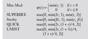
Some of them are mentioned below

Van Leer flux limiter function = `(r+|r|)/(1+r)`

Van Albada flux limiter function = `(r+r^2)/(1+r^2)`