Week 5 - Mid term project - Solving the steady and unsteady 2D heat conduction problem
2D Heat conduction equation:
`(delT)/(delt) = alpha*((del^2T)/(delx^2)+ (del^2T)/(dely^2))` --> (1)
whre T is temperature; t is time, `alpha`is thermal diffusivity
Eq. (1) is unsteady state heat conduction in which the temperature varies with respect to time and space.
For a steady flow heat conduction, temperature does not vary with time instead only varies with space.
So, eq. (1) becomes
`(del^2T)/(delx^2) + (del^2T)/(dely^2) = 0` --> (2)
The unsteady equation (1) is a hyperbolic PDE and can be solved using time marching technique. So, the equation can be discretized explicitly or implicitly.
For explicit approach, as there will be only one unknown term in a equation, it can be solved without much complication.
But for implicit method, as there are more unknown terms in an equation, it is generally solved by doing matrix inversions. This is feasible if the domain has less no. of elements, but in real world applications, the mesh contains lakhs of elements. To create a matrix with these many values takes up more space and time. In order to solve these equations, iterative solvers are used.
Consider system of linear equations given by matrices AX = B where X is the solution. A and B are knowns.
These iterative solvers initially assume a random guess solution (random X vector) to the problem and calculates the difference between the actual known B and B obtained by random X. This difference is called Residual. If this difference is less than a given defined value, then the random X is the final solution otherwise based on the residual, another random X is estimated and the process goes on until it satsifies a given criteria. This method is called Fixed Point method.
The iterative solvers are of three types:
1. Jacobi
2. Gauss-Siedel
3. Successive Over Relaxation (SOR)
Now, these three solvers are used to solve the steady and unsteady equations and are compared to find out which solver computes faster.
Steady State Equation:
The above three iterative solvers are used to solve the steady state equation and are compared to find out which solver computes faster.
Equation (2) is discretized with central differencing scheme as follows
let `T_(i,j)` be the temperature at 'i' th row and 'j' th column.
`(T_(i-1,j) - 2*T_(i,j) + T_(i+1,j))/dx^2 + (T_(i,j-1) - 2*T_(i,j) + T_(i,j+1))/dy^2 = 0` --> (3)
let
`T_(i,j)` = temperature at point P
`T_(i-1,j)` = temperature at the left node of point P = `T_L`
`T_(i+1,j)` = temperature at the right node of point P = `T_R`
`T_(i,j-1)` = temperature at the top node of point P = `T_T`
`T_(i,j+1)`= temperature at the bottom node of point P = `T_B`
Therefore,
`(T_L - 2*T_P + T_R)/dx^2 + (T_T - 2*T_P + T_B)/dy^2 = 0` --> (4)
Solving for `T_P`, we get
`T_P = (1/K)*((T_L + T_R)/dx^2 + (T_T + T_B)/dy^2)` --> (5)
where
k = `2*((dx^2 + dy^2)/(dx^2*dy^2))`
Unsteady state Equation:
Equation (1) is discretized with first order forward difference for unsteady term and central difference scheme for spatial terms.
let
`T_(i,j)^n` = temperature at point at time 'n'`
`T_(i,j)^(n+1)` = temperature at point at time 'n+1'`
`T_(i-1,j)^n` = temperature at the left node of point P at time 'n' = `T_L^n`
`T_(i+1,j)^n` = temperature at the right node of point P at time 'n' = `T_R^n`
`T_(i,j-1)^n` = temperature at the top node of point P at time 'n' = `T_T^n`
`T_(i,j+1)^n`= temperature at the bottom node of point P at time 'n'= `T_B^n`
`T_(i-1,j)^(n+1)` = temperature at the left node of point P at time 'n+1' = `T_L^(n+1)`
`T_(i+1,j)^(n+1)` = temperature at the right node of point P at time 'n+1' = `T_R^(n+1)`
`T_(i,j-1)^(n+1)` = temperature at the top node of point P at time 'n+1' = `T_T^(n+1)`
`T_(i,j+1)^(n+1)`= temperature at the bottom node of point P at time 'n+1'= `T_B^(n+1)`
Explicit approach:
The unsteady equation using explicit approach is solved directly without using iterative solvers. This generally does not take much time nor does it occupy much space as the equations are direct with only one unknown and rest of the terms are known.
`(T_(i,j)^(n+1) - T_(i,j)^n)/dt = alpha*( (T_(i-1,j)^n - 2*T_(i,j)^n + T_(i+1,j)^n)/dx^2 + (T_(i,j-1)^n - 2*T_(i,j)^n + T_(i,j+1)^n)/dy^2)` -->(6)
It can be written as
`(T_p^(n+1) - T_P^n)/dt = alpha*((T_L^n - 2*T_P^n + T_R^n)/dx^2 + (T_T^n - 2*T_P^n + T_B^n)/dy^2)`
Solving for `T_P^(n+1)`, we get
`T_p^(n+1) = T_P^n + k1*(T_L^n - 2*T_P^n + T_R^n) + k2*(T_T^n - 2*T_P^n + T_B^n)` -->(7)
where `k1 = (alpha*dt)/dx^2 ; k2 = (alpha*dt)/dy^2`
For the explicit approach to be stable, it must satisfy the CFL condition.
The CFL condition is
`(k1 + k2) <= 0.5`
From this, dt is obtained as
`dt = 0.5/((alpha/dx^2) + (alpha/dy^2)` -->(8)
Implicit approach:
The above three iterative solvers are used to solve the steady state equation and are compared to find out which solver computes faster.
`(T_(i,j)^(n+1) - T_(i,j)^n)/dt = alpha*( (T_(i-1,j)^(n+1) - 2*T_(i,j)^(n+1) + T_(i+1,j)^(n+1))/dx^2 + (T_(i,j-1)^(n+1) - 2*T_(i,j)^(n+1) + T_(i,j+1)^(n+1))/dy^2)` --> (9)
It can be written as
`(T_p^(n+1) - T_P^n)/dt = alpha*((T_L^(n+1) - 2*T_P^(n+1) + T_R^(n+1))/dx^2 + (T_T^(n+1) - 2*T_P^(n+1) + T_B^(n+1))/dy^2)`
Solving for `T_P^(n+1)`, we get
`T_p^(n+1) = T_P^n + k1*(T_L^(n+1) - 2*T_P^(n+1) + T_R^(n+1)) + k2*(T_T^(n+1) - 2*T_P^(n+1) + T_B^(n+1))`
where `k1 = (alpha*dt)/dx^2 ; k2 = (alpha*dt)/dy^2`
Further solving,
`T_P^(n+1) = (T_P^n + k1*(T_L^(n+1) + T_R^(n+1)) + k2*(T_T^(n+1) + T_B^(n+1)))/((1 + 2*k1 + 2*k2))` ---> (10)
Further simplifying,
`T_P^(n+1) = (term1*T_P^n) + (term2*(T_L^(n+1) + T_R^(n+1))) + (term3*(T_T^(n+1) + T_B^(n+1)))` --> (11)
`T_P^(n+1) = (term1*T_P^n) + (term2*H) + (term3*V)` ` --> (12)
where
term1 = (1 + 2*k1 +2*k2)
term2 = k1 * term1
term3 = k2 * term1
H = `(T_L^(n+1) + T_R^(n+1))`
V = `(T_T^(n+1) + T_B^(n+1))`
MATLAB Codes:
1. Main Program:
Given initial conditions are
T at top boundary = 600 k
T at bottom boundary = 900 k
T at left boundary = 400 K
T at right boundary = 800 K
% Week 5 Challenge 1
% 2D steady and unsteady state heat conduction
% given BCs are T_top = 600; T_bottom = 900; T_left = 400; T_right = 800

clear all
close all
clc

nx = 10;
ny = 10;
l = 1;
b = 1;
x = linspace(0,l,nx);
y = linspace(0,b,ny);
dx = l/(nx-1);
dy = b/(ny-1);
tol = 1e-4;
w = 1.2;
a = 1.5;

T_old = 300*ones(nx,ny);
T_old(1,1) = 500;
T_old(1,nx) = 700;
T_old(ny,1) = 650;
T_old(nx,ny) = 850;
T_old(2:end-1,1) = 400;
T_old(1,2:end-1) = 600;
T_old(2:end-1,end) = 800;
T_old(end,2:end-1) = 900;

dt = 0.5/((a/dx^2) + (a/dy^2));

%Steady State d^2x/dt^2 = 0

% Jacobi Solver
[T_st_j, Jacobi_iteration_st] = steady_state_Jacobi(T_old,nx,ny,l,b,tol);

% Gauss-Siedel Solver
[T_st_gs, Gauss_iteration_st] = steady_state_Gauss(T_old,nx,ny,l,b,tol);

% SOR solver
[T_st_sor, SOR_iteration_st] = steady_state_SOR(T_old,nx,ny,l,b,tol,w);


%Unsteady State dT/dt = a*((d^2x/dt^2) + (d^2x/dt^2))

% Explicit
[T_un_exp, explicit_iteration_un] = unsteady_explicit(T_old,nx,ny,l,b,a,tol);

%Implicit - Jacobi
[T_un_j, Jacobi_iteration_un] = unsteady_Jacobi(T_old,nx,ny,l,b,a,dt,tol);

% Implicit - Gauss-Siedel
[T_un_gs, Gauss_iteration_un] = unsteady_Gauss(T_old,nx,ny,l,b,a,dt,tol);

% Implicit - SOR with Gauss-Siedel
[T_un_sor, SOR_iteration_un] = unsteady_SOR(T_old,nx,ny,l,b,a,dt,tol,w);

%plots
figure(8)
contourf(T_old)
colorbar; colormap(jet);
axis ij
axis equal
grid on
title_text1 = sprintf('Initial conditions');
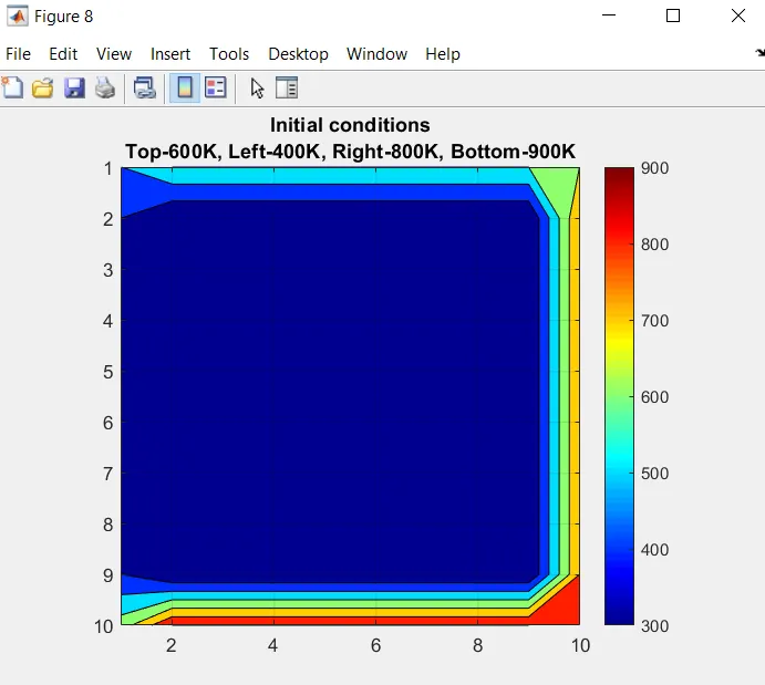
title_text2 = sprintf('Top-600K, Left-400K, Right-800K, Bottom-900K');
title({(title_text1), (title_text2)});

figure(9)
steady_iterations = [Jacobi_iteration_st Gauss_iteration_st SOR_iteration_st];
x = categorical({'Jacobi', 'Gauss-Siedel', 'SOR with G-S'});
bar(x,steady_iterations);
xlabel('Iterative Solver Method');
ylabel('No. of iterations');
title('Steady State-No. of iterations by various iterative solvers');

figure(10)
unsteady_iterations = [explicit_iteration_un Jacobi_iteration_un Gauss_iteration_un SOR_iteration_un];
x = categorical({'Explicit', 'Jacobi', 'Gauss-Siedel', 'SOR with G-S'});
bar(x,unsteady_iterations);
xlabel('Iterative Solver Method');
ylabel('No. of iterations');
title('Unsteady State-No. of iterations by various iterative solvers');
The domain here is considered to be a square of length(l) = 1m and breadth(b) = 1m
Domain is divided into a grid of 100 elements by giving no. of nodes in X-direction (nx) = 10 and no. of nodes in Y-direction (ny) = 10
Each node is seperated by a fixed distance in X and Y direction
dx = l/(n-1) and dy = b/(n-1)
The error criteria to which the solver must converge is given by 'tol' = 1e-4.
Thermal diffusivity (a) value is assumed to be 1.5.
Relaxation factor (w) is assumed to be 1.2.
Time step size is given by eq. (8) and is taken same for both explicit and implicit approaches.
Initially, a random solution for T is estimated and given by 'T_old'.
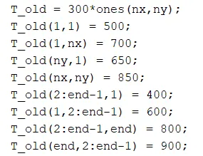
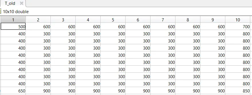
A contour for T_old is generated with initial conditions
Functions are written for steady and unsteady cases and written in the main program.
Two bar graphs(Figure 9 & 10) one for steady state and another for unsteady are generated to compare the no. of iterations taken by each solver.
2. Steady State solvers:
(i) Function for solving steady state equation using Jacobi iterative solver:
Let `T_P^m`be the temperature at point P at 'm'th iteration. Based on the central differencing scheme, the tempearture at P is calculated considering the temperatures at the surrounding nodes. In the Jacobi method, temp. at P at '(m+1)' th iteration is calculated considering temperatures of surrounding nodes of 'm'th iteration until the solution converges.
equation (5) for Jacobi method will be of the form
`T_P^(m+1) = (1/K)*((T_L^m + T_R^m)/dx^2 + (T_T^m + T_B^m)/dy^2)``
% Week 5 Challenge 1
% Function for 2D steady state heat conduction solving with Jacobi solver
% d^T/dx^2 + d^T/dy^2 = 0
% given inputs are T_top = 600; T_bottom = 900; T_left = 400; T_right = 80

function[T_st_j, Jacobi_iteration_st] = steady_state_Jacobi(T_old,nx,ny,l,b,tol)

dx = l/(nx-1);
dy = b/(ny-1);
error = 9e9;

T_st_j = T_old;

k = (2*(dx^2 + dy^2))/(dx^2 * dy^2);

Jacobi_iteration_st = 1;

while (error > tol)

for j = 2:(ny-1)
    for i = 2:(nx-1)

        term1 = (T_old(i+1,j) + T_old(i-1,j))/(k * (dx^2));
        term2 = (T_old(i,j-1) + T_old(i,j+1))/(k * (dy^2));

        T_st_j(i,j) = term1 + term2;
    end
end

error = max(max(abs(T_old - T_st_j)));
T_old = T_st_j;
Jacobi_iteration_st = Jacobi_iteration_st + 1;

figure(1)
contourf(T_st_j);
axis ij;
grid on;
colorbar; colormap(jet);
title_text1 = sprintf('Steady State : Jacobi Solver, iteration number = %d', Jacobi_iteration_st);
title_text2 = sprintf('Max. temperature difference = %f', error);
title({[title_text1],[title_text2]});
pause(0.003);

end

end
The function takes inputs as T_old, nx, ny, l, b, tol which are defined in the main program.
Initially, temperatures T_old is stored in another matrix 'T_st_j'.
The error value is given as 9e9 to enter the while loop.
Two for loops one for X direction and another for Y direction are written to calculate temperatures at all nodes.
Then, the error between calculated temperatures 'T_st_j' and temperatured at previous iteration 'T_old' is calculated and if this converges i.e., if the error value is less than a partilcular criteria, the solver exits while loop and final T values are obtained. If the error value does not satisfy the criteria, 'T_st_j' values are copied into T_old and another iteration carries on to calculate new 'T_st_j'.
No. of iterations are also calculated as 'Jacobi_iteration_st' and is incremented after each iteration.
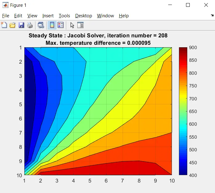
A contour is generated for each iteration until the solver attains staedy state.
(ii) Function for solving steady state equation using Gauss-Siedel iterative solver:
Let `T_P^m`be the temperature at point P at 'm'th iteration. Based on the central differencing scheme, the temperature at P is calculated considering the temperatures at the surrounding nodes. In the Gauss-Siedel method, temp. at P at '(m+1)' th iteration is calculated considering temperatures of surrounding nodes of that current '(m+1)'th if available or if not availabe, ir considers temperatures at 'm' th iteration until the solution converges.
equation (5) for Gauss-Siedel method will be of the form
`T_P^(m+1) = (1/K)*((T_L^(m+1) + T_R^m)/dx^2 + (T_T^(m+1) + T_B^m)/dy^2)``
% Week 5 Challenge 1
% Function for 2D steady state heat conduction solving with Gauss-siedel solver
% d^T/dx^2 + d^T/dy^2 = 0
% given inputs are T_top = 600; T_bottom = 900; T_left = 400; T_right = 80

function[T_st_gs, Gauss_iteration_st] = steady_state_Gauss(T_old,nx,ny,l,b,tol)

dx = l/(nx-1);
dy = b/(ny-1);
error = 9e9;

T_st_gs = T_old;

k = (2*(dx^2 + dy^2))/(dx^2 * dy^2);

Gauss_iteration_st = 1;

while (error > tol)

for j = 2:(ny-1)
    for i = 2:(nx-1)

        term1 = (T_old(i+1,j) + T_st_gs(i-1,j))/(k * (dx^2));
        term2 = (T_st_gs(i,j-1) + T_old(i,j+1))/(k * (dy^2));

        T_st_gs(i,j) = term1 + term2;

    end
end

error = max(max(abs(T_old - T_st_gs)));
T_old = T_st_gs;
Gauss_iteration_st = Gauss_iteration_st + 1;

figure(2)
contourf(T_st_gs);
axis ij;
grid on;
colorbar; colormap(jet);
title_text1 = sprintf('Steady State : Gauss Siedel Solver, iteration number = %d', Gauss_iteration_st);
title_text2 = sprintf('Max. temperature difference = %f', error);
title({[title_text1],[title_text2]});
pause(0.003);

end

end
The function takes inputs as T_old, nx, ny, l, b, tol which are defined in the main program.
Initially, temperatures T_old is stored in another matrix 'T_st_gs'.
The error value is given as 9e9 to enter the while loop.
Two for loops one for X direction and another for Y direction are written to calculate temperatures at all nodes.
Then, the error between calculated temperatures 'T_st_gs' and temperature at previous iteration 'T_old' is calculated and if this converges i.e., if the error value is less than a partilcular criteria, the solver exits while loop and final T values are obtained. If the error value does not satisfy the criteria, 'T_st_gs' values are copied into T_old and another iteration carries on to calculate new 'T_st_gs'.
No. of iterations are also calculated as 'Gauss_iteration_st' and is incremented after each iteration.
A contour is generated for each iteration until the solver attains steady state.
(iii) Function for solving steady state equation using SOR iterative solver:
The SOR method is an enhanced method compared to Jacobi and Gauss Siedel, It introduces a variable called relaxation factor (w) to converge the solution faster compared to preious iterative solvers. Also, if w value is greater than 1, the solution converges faster.
equation (5) for SOR method will be of the form
`T_P^(m+1) = (1-w)*T_P^(m) + (w/K)*((T_L^(m+1) + T_R^m)/dx^2 + (T_T^(m+1) + T_B^m)/dy^2)``
% Week 5 Challenge 1
% Function for 2D steady state heat conduction solving with SOR solver
% d^T/dx^2 + d^T/dy^2 = 0
% given inputs are T_top = 600; T_bottom = 900; T_left = 400; T_right = 80

function[T_st_sor, SOR_iteration_st] = steady_state_SOR(T_old,nx,ny,l,b,tol,w)

dx = l/(nx-1);
dy = b/(ny-1);
error = 9e9;

T_st_sor = T_old;

k = (2*(dx^2 + dy^2))/(dx^2 * dy^2);

SOR_iteration_st = 1;

while (error > tol)

for j = 2:(ny-1)
    for i = 2:(nx-1)

        term1 = (T_old(i+1,j) + T_st_sor(i-1,j))/(k * (dx^2));
        term2 = (T_st_sor(i,j-1) + T_old(i,j+1))/(k * (dy^2));
        term3 = (1-w)*T_old(i,j);
        T_st_sor(i,j) = term3 + w*(term1 + term2);
    end
end

error = max(max(abs(T_old - T_st_sor)));
T_old = T_st_sor;
SOR_iteration_st = SOR_iteration_st + 1;

figure(3)
contourf(T_st_sor);
axis ij;
grid on;
colorbar; colormap(jet);
title_text1 = sprintf('Steady State : SOR Solver, iteration number = %d', SOR_iteration_st);
title_text2 = sprintf('Max. temperature difference = %f', error);
title({[title_text1],[title_text2]});
pause(0.003);

end

end
The function takes inputs as T_old, nx, ny, l, b, tol, w which are defined in the main program.
Initially, temperatures T_old is stored in another matrix 'T_st_sor'.
The error value is given as 9e9 to enter the while loop.
Two for loops one for X direction and another for Y direction are written to calculate temperatures at all nodes.
Then, the error between calculated temperatures 'T_st_sor' and temperature at previous iteration 'T_old' is calculated and if this converges i.e., if the error value is less than a partilcular criteria, the solver exits while loop and final T values are obtained. If the error value does not satisfy the criteria, 'T_st_sor' values are copied into T_old and another iteration carries on to calculate new 'T_st_sor'.
No. of iterations are also calculated as 'SOR_iteration_st' and is incremented after each iteration.
A contour is generated for each iteration until the solver attains steady state.
3. Unsteady State Solvers:
Here, temperature also changes with respect to time and the time taken to solve the equation is also found out.
(i) Explicit approach:
The explicit approach does not need iterative solvers to solve the governing equation as there is only one unknown in each equation of the node.
A guess value is estimated initially for first time step and temperature is obtained at next time step considering the guess value. The temperature difference beween the old and new value is calculated and if this is greater than a given value, temperature for next time step is calculated. If the temp. difference is less than that particular value, steady state is achieved.
For this purpose, a while loop is created as "while (max_temp_diff > tol)". For each time step, the code calculates the max. temp. difference and if that values is less than tol, the while loop is exited otherwise it keeps on iterating until the condition is satisfied.
max temp. difference is iniially given a value of 9e9 to enter the while loop.
No. of iterations, no. of time steps and total time the code takes to obtain steady state is also calculated.
time step size value 'dt' is obtained by eq. (8).
Time steps and no. of iterations are incremented each time whenever the while loop condition is not satisfied and the code enters the while loop.
Time is obtained by multiplying the dt value with time step.
% Week 5 Challenge 1
% Function for 2D unsteady state heat conduction solving explicitly
% dT/dt = a*(d^T/dx^2 + d^T/dy^2)
% given BCs are T_top = 600; T_bottom = 900; T_left = 400; T_right = 80

function[T_un_exp, explicit_iteration_un] = unsteady_explicit(T_old,nx,ny,l,b,a,tol)

dx = l/(nx-1);
dy = b/(ny-1);

T_un_exp = T_old;

dt = 0.5/((a/dx^2) + (a/dy^2));

k1 = (a*dt)/(dx^2);
k2 = (a*dt)/(dy^2);

time_step = 1;
max_temp_diff = 9e9;
explicit_iteration_un = 1;

while(max_temp_diff > tol)
    time = dt*time_step;

    for j = 2:(ny-1)
        for i = 2:(nx-1)

            term1 = k1*(T_old(i-1,j) - 2*(T_old(i,j)) + T_old(i+1,j));
            term2 = k2*(T_old(i,j-1) - 2*(T_old(i,j)) + T_old(i,j+1));

            T_un_exp(i,j) = T_old(i,j) + term1 + term2;

        end
    end
    max_temp_diff = max(max(abs(T_old - T_un_exp)));

    T_old = T_un_exp;
    time_step = time_step + 1;
    explicit_iteration_un = explicit_iteration_un + 1;

figure(4)
contourf(T_un_exp);
axis ij;
grid on;
colorbar; colormap(jet);
title_text1 = sprintf('Unsteady State : Explicit, Time step = %d', time_step);
title_text2 = sprintf('Max. Temperature difference = %f', max_temp_diff);
title_text3 = sprintf('Time = %f', time);
title_text4 = sprintf('Iterations = %d', explicit_iteration_un);
title({(title_text1),(title_text2),(title_text3),(title_text4)});
pause(0.003);

end

end
The function takes inputs as T_old, nx, ny, l, b, a, tol.
Initially, temperatures T_old is stored in another matrix 'T_un_exp'.
Two for loops one for X direction and another for Y direction are written to calculate temperatures at all nodes.
No. of iterations are calculated as 'explicit_iteration_un' and is incremented after each iteration.
A contour is generated for each iteration (time step) until the solver attains steady state.
(ii) Implicit - Function for solving unsteady state equation implicitly using Jacobi iterative solver:
let `T_P^(n,m)` be the temperature at node P at time 'n' and 'm' th iteration.
Based on the central differencing scheme, the tempearture at P is calculated considering the temperatures at the surrounding nodes. In this method, at a particular time, temp. at P at '(m+1)' th iteration is calculated considering temperatures of surrounding nodes of 'm'th iteration until the solution converges.
Eq. (11) for Jacobi method will be of the form
`T_P^((n+1),(m+1)) = (term1*T_P^n) + (term2*(T_L^((n+1),m) + T_R^((n+1),m))) + (term3*(T_T^((n+1),m) + T_B^((n+1),m)))` `
% Week 5 Challenge 1
% Function for 2D unsteady state heat conduction solving implicitly -
% Jacobi
% dT/dt = a*(d^T/dx^2 + d^T/dy^2)
% given BCs are T_top = 600; T_bottom = 900; T_left = 400; T_right = 80

function[T_un_j, Jacobi_iteration_un] = unsteady_Jacobi(T_old,nx,ny,l,b,a,dt,tol)

dx = l/(nx-1);
dy = b/(ny-1);

T_un_j = T_old;
T_prev = T_old;

k1 = (a*dt)/(dx^2);
k2 = (a*dt)/(dy^2);

term1 = 1/(1+(2*k1)+(2*k2));
term2 = k1*term1;
term3 = k2*term1;

time_step = 1;
Jacobi_iteration_un = 1;
max_temp_diff = 9e9;

while(max_temp_diff > tol)
    error = 9e9;
    time = dt*time_step;
    while (error > tol)
         for j = 2:(ny-1)
             for i = 2:(nx-1)

                 H = (T_old(i-1,j) + T_old(i+1,j));
                 V = (T_old(i,j-1) + T_old(i,j+1));

                 T_un_j(i,j) = (term1*T_prev(i,j)) + (term2*H) + (term3*V);
             end
         end
         error = max(max(abs(T_old - T_un_j)));
         T_old = T_un_j;
         Jacobi_iteration_un = Jacobi_iteration_un + 1;
    end
     max_temp_diff = max(max(abs(T_prev - T_un_j)));
     T_prev = T_un_j;
     time_step = time_step + 1;

figure(5)
contourf(T_un_j);
axis ij;
grid on;
colorbar; colormap(jet);
title_text1 = sprintf('Unsteady State : Implicit-Jacobi, Time step = %d', time_step);
title_text2 = sprintf('Max. Temperature difference = %f', max_temp_diff);
title_text3 = sprintf('Iterations = %d', Jacobi_iteration_un);
title_text4 = sprintf('Time = %f', time);
title({(title_text1),(title_text2),(title_text3),(title_text4)});
pause(0.003);

end
A guess value is estimated initially for first time step. The steady state is obtained with two steps.
In step 1, the code takes the initial guess value and obtains a next best guess value by solving iteratively using Jacobi method i.e., for the first time step, the code computes a next best guess value and calculates the error bewteen old and new guess value. If this error satisfies a particular condition, the iteration is complete and temperature at next time step is obtained.
For this purpose, a while loop is created "while (error > tol)". The governing equation is written inside this while loop in the form mentioned above and temp. at next time step is obtained.
In step 2, temperarture difference between time step 1 and time step 2 is calculated and if it is less than max. temp. difference allowed, steady state is obtained. If not, temperatures at next time steps is obtained as described in step 1. Thsi process continues until the steady state is obtained.
For this purpose, another while loop "while (max_temp_diff > tol)" is created.
Initially, T_old is copied into T_prev and T_un_j.
T_old is the temperature at pevious iteration whereas T_prev is the temperature at previous time step.
T_old keeps on changing in the step 1 whereas T_prev remains constant in step 1.
No. of iterations the Jacobi solver takes for solving is calculated by writing "Jacobi_iteration_un = Jacobi_iteration_un + 1" in step 1.
No. of time steps and total time in whicg steady state is obtained is calculated by writing "time_step = time_step + 1" and "time = dt*time_step" in step 2.
A contour is generated at each time step till the steady state is reached.
(iii) Implicit - Function for solving unsteady state equation implicitly using Gauss-Siedel iterative solver:
let `T_P^(n,m)` be the temperature at node P at time 'n' and 'm' th iteration.
Based on the central differencing scheme, the tempearture at P is calculated considering the temperatures at the surrounding nodes. In the Gauss-Siedel method, at a particular time, temp. at P at '(m+1)' th iteration is calculated considering temperatures of surrounding nodes of that current '(m+1)'th if available or if not availabe, ir considers temperatures at 'm' th iteration until the solution converges.
Eq. (11) for Gauss-Siedel method will be of the form
`T_P^((n+1),(m+1)) = (term1*T_P^n) + (term2*(T_L^((n+1),(m+1)) + T_R^((n+1),m))) + (term3*(T_T^((n+1),(m+1)) + T_B^((n+1),m)))` `
% Week 5 Challenge 1
% Function for 2D unsteady state heat conduction solving implicitly -
% Gauss-Siedel
% dT/dt = a*(d^T/dx^2 + d^T/dy^2)
% given BCs are T_top = 600; T_bottom = 900; T_left = 400; T_right = 80

function[T_un_gs, Gauss_iteration_un] = unsteady_Gauss(T_old,nx,ny,l,b,a,dt,tol)

dx = l/(nx-1);
dy = b/(ny-1);

T_un_gs = T_old;
T_prev = T_old;

k1 = (a*dt)/(dx^2);
k2 = (a*dt)/(dy^2);

term1 = 1/(1+(2*k1)+(2*k2));
term2 = k1*term1;
term3 = k2*term1;

time_step = 1;
Gauss_iteration_un = 1;
max_temp_diff = 9e9;

while(max_temp_diff > tol)
    error = 9e9;
    time = dt*time_step;
    while (error > tol)
         for j = 2:(ny-1)
             for i = 2:(nx-1)

                 H = (T_un_gs(i-1,j) + T_old(i+1,j));
                 V = (T_un_gs(i,j-1) + T_old(i,j+1));

                 T_un_gs(i,j) = (term1*T_prev(i,j)) + (term2*H) + (term3*V);
             end
         end
         error = max(max(abs(T_old - T_un_gs)));
         T_old = T_un_gs;
         Gauss_iteration_un = Gauss_iteration_un + 1;
    end
     max_temp_diff = max(max(abs(T_prev - T_un_gs)));
     T_prev = T_un_gs;
     time_step = time_step + 1;

figure(6)
contourf(T_un_gs);
axis ij;
grid on;
colorbar; colormap(jet);
title_text1 = sprintf('Unsteady State : Implicit-Gauss Siedel, Time step = %d', time_step);
title_text2 = sprintf('Max. Temperature difference = %f', max_temp_diff);
title_text3 = sprintf('Iterations = %d', Gauss_iteration_un);
title_text4 = sprintf('Time = %f', time);
title({(title_text1),(title_text2),(title_text3),(title_text4)});
pause(0.003);

end
A guess value is estimated initially for first time step. The steady state is obtained with two steps.
In step 1, the code takes the initial guess value and obtains a next best guess value by solving iteratively using Gauss-Siedel method i.e., for the first time step, the code computes a next best guess value and calculates the error bewteen old and new guess value. If this error satisfies a particular condition, the iteration is complete and temperature at next time step is obtained.
For this purpose, a while loop is created "while (error > tol)". The governing equation is written inside this while loop in the form mentioned above and temp. at next time step is obtained.
In step 2, temperarture difference between time step 1 and time step 2 is calculated and if it is less than max. temp. difference allowed, steady state is obtained. If not, temperatures at next time steps is obtained as described in step 1. Thsi process continues until the steady state is obtained.
For this purpose, another while loop "while (max_temp_diff > tol)" is created.
Initially, T_old is copied into T_prev and T_un_gs.
T_old is the temperature at pevious iteration whereas T_prev is the temperature at previous time step.
T_old keeps on changing in the step 1 whereas T_prev remains constant in step 1.
No. of iterations the Gauss solver takes for solving is calculated by writing "Gauss_iteration_un = Gauss_iteration_un + 1" in step 1.
No. of time steps and total time in whicg steady state is obtained is calculated by writing "time_step = time_step + 1" and "time = dt*time_step" in step 2.
A contour is generated at each time step till the steady state is reached.
(iv) Implicit - Function for solving unsteady state equation implicitly using SOR iterative solver:
let `T_P^(n,m)` be the temperature at node P at time 'n' and 'm' th iteration.
The SOR method is an enhanced method compared to Jacobi and Gauss Siedel, It introduces a variable called relaxation factor (w) to converge the solution faster compared to preious iterative solvers. Also, if w value is greater than 1, the solution converges faster.
Eq. (11) for SOR method will be of the form
`T_P^((n+1),(m+1)) = (1-w)*T_P^(n+1,m) + w*((term1*T_P^n) + (term2*(T_L^((n+1),(m+1)) + T_R^((n+1),m))) + (term3*(T_T^((n+1),(m+1)) + T_B^((n+1),m))))` `
% Week 5 Challenge 1
% Function for 2D unsteady state heat conduction solving implicitly -
% SOR
% dT/dt = a*(d^T/dx^2 + d^T/dy^2)
% given BCs are T_top = 600; T_bottom = 900; T_left = 400; T_right = 80

function[T_un_sor, SOR_iteration_un] = unsteady_SOR(T_old,nx,ny,l,b,a,dt,tol,w)

dx = l/(nx-1);
dy = b/(ny-1);

T_un_sor = T_old;
T_prev = T_old;

k1 = (a*dt)/(dx^2);
k2 = (a*dt)/(dy^2);

term1 = 1/(1+(2*k1)+(2*k2));
term2 = k1*term1;
term3 = k2*term1;

time_step = 1;
SOR_iteration_un = 1;
max_temp_diff = 9e9;

while(max_temp_diff > tol)
    error = 9e9;
    time = dt*time_step;
    while (error > tol)
         for j = 2:(ny-1)
             for i = 2:(nx-1)

                 H = (T_un_sor(i-1,j) + T_old(i+1,j));
                 V = (T_un_sor(i,j-1) + T_old(i,j+1));
                 term4 = (1-w)*T_old(i,j);
                 T_un_sor(i,j) = term4 + w*((term1*T_prev(i,j)) + (term2*H) + (term3*V));
             end
         end
         error = max(max(abs(T_old - T_un_sor)));
         T_old = T_un_sor;
         SOR_iteration_un = SOR_iteration_un + 1;
    end
     max_temp_diff = max(max(abs(T_prev - T_un_sor)));
     T_prev = T_un_sor;
     time_step = time_step + 1;

figure(7)
contourf(T_un_sor);
axis ij;
grid on;
colorbar; colormap(jet);
title_text1 = sprintf('Unsteady State : Implicit-SOR, Time step = %d', time_step);
title_text2 = sprintf('Max. Temperature difference = %f', max_temp_diff);
title_text3 = sprintf('Iterations = %d', SOR_iteration_un);
title_text4 = sprintf('Time = %f', time);
title({(title_text1),(title_text2),(title_text3),(title_text4)});
pause(0.003);

end
A guess value is estimated initially for first time step. The steady state is obtained with two steps.
In step 1, the code takes the initial guess value and obtains a next best guess value by solving iteratively using SOR method i.e., for the first time step, the code computes a next best guess value and calculates the error bewteen old and new guess value. If this error satisfies a particular condition, the iteration is complete and temperature at next time step is obtained.
For this purpose, a while loop is created "while (error > tol)". The governing equation is written inside this while loop in the form mentioned above and temp. at next time step is obtained.
In step 2, temperarture difference between time step 1 and time step 2 is calculated and if it is less than max. temp. difference allowed, steady state is obtained. If not, temperatures at next time steps is obtained as described in step 1. This process continues until the steady state is obtained.
For this purpose, another while loop "while (max_temp_diff > tol)" is created.
Initially, T_old is copied into T_prev and T_un_sor.
T_old is the temperature at pevious iteration whereas T_prev is the temperature at previous time step.
T_old keeps on changing in the step 1 whereas T_prev remains constant in step 1.
No. of iterations the Gauss solver takes for solving is calculated by writing "SOR_iteration_un = SOR_iteration_un + 1" in step 1.
No. of time steps and total time in which steady state is obtained is calculated by writing "time_step = time_step + 1" and "time = dt*time_step" in step 2.
A contour is generated at each time step till the steady state is reached.
Outputs:
Contours for steady and transient states are generated showing the temperature distribution across the domain along with the no. of iterations and time steps a particular solver took to complete.
1. Steady State:
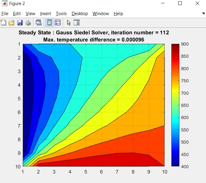
(i) Jacobi:
(ii) Gauss-Siedel:
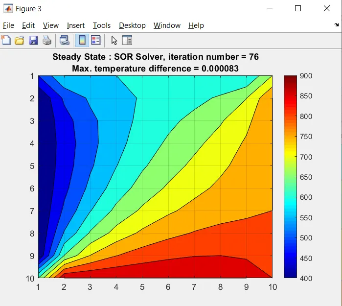
(iii) SOR:
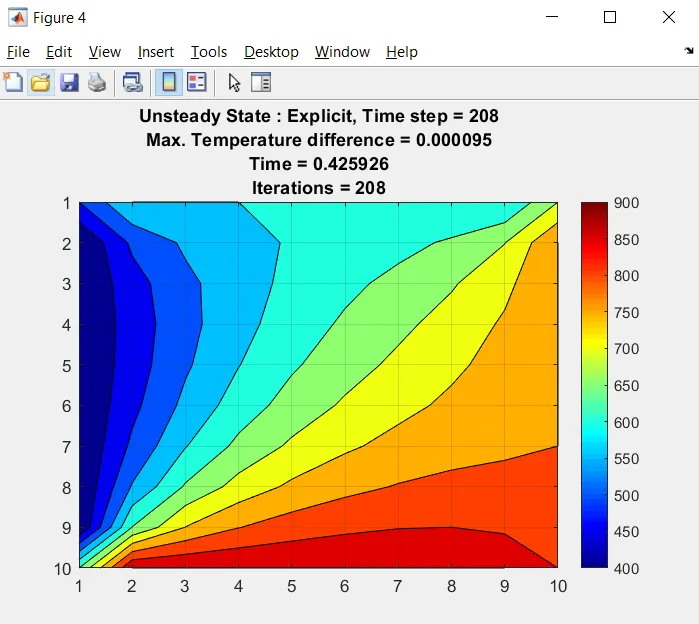
2. Unsteady State:
(i) Explicit:
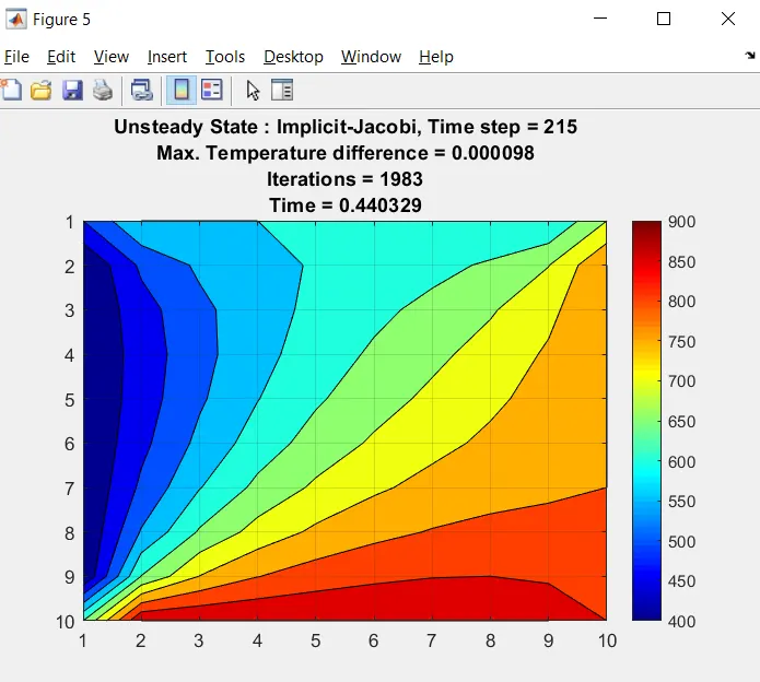
(ii) Implicit - Jacobi:
(iii) Implicit - Gauss-Siedel:
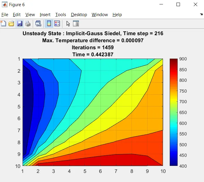
(iv) Implicit - SOR:
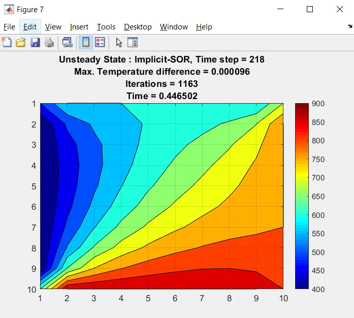
3. Comparing the no.of iterations taken by each solver:
(i) Steady State:
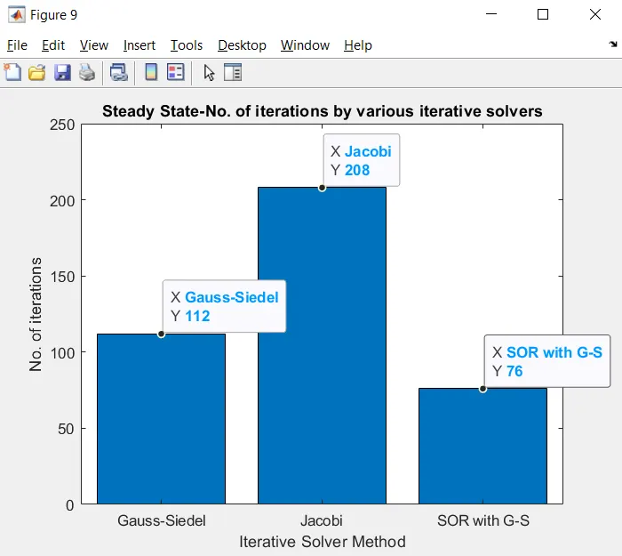
(ii) Unsteady state:
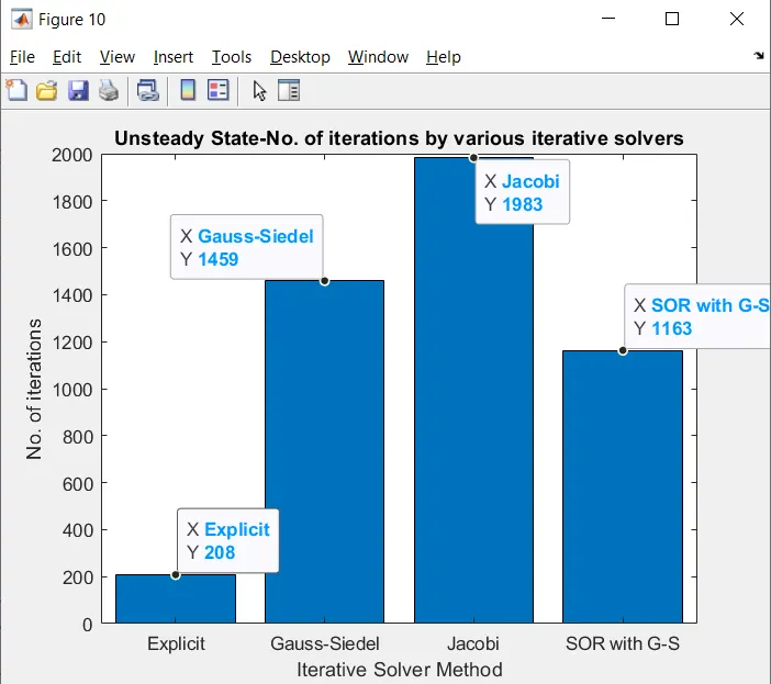
Conclusions:
1. Steady state:
From the above plots, it is observed that
The Jacobi solver iterates 208 times to solve the problem (to converge).
Gauss-Siedel iterates 112 times to converge. It is almost 50% less than Jacobi.
SOR solver iterates only 76 times to converge. It is almost 65% less than Jacobi and almost 30% less than Gauss-Siedel.
(No. of iterations Jacobi takes) > (No. of iterations Gauss Siedel takes) > (No. of iterations SOR takes).
That means, for solving a same problem, SOR solver takes 65% less time to solve compared to Jacobi and 30% less time compared to Gauss-Siedel.
2. Unsteady State:
For implicit,
The Jacobi solver iterates 1983 times to solve the problem (to converge).
Gauss-Siedel iterates 1459 times to converge. It is almost 25% less than Jacobi.
SOR solver iterates 1163 times to converge. It is almost 40% less than Jacobi and almost 20% less than Gauss-Siedel.
Solving the problem using explicit approach takes just 208 iterations.
(No. of iterations Jacobi takes) > (No. of iterations Gauss Siedel takes) > (No. of iterations SOR takes) > (Solving by explicit approach).
As mentioned in the start, explicit approach is a direct approach wherein there is only one unknown but the drawback is, it is conditionally stable i.e., if the equation (8) is not satisfied, the solution blows up.
The time step size used to calculate the above problem is 0.002057. Suppose, in a particular application governed by the (2) eq., if the time step size needs to be more than 0.002057, the solution will be unstable.
Whereas the implicit approach is unconditionally stable i.e, the solution will be stable for any value of time step. So, a bigger time step can be taken which can solve the problem in fewer time steps.
With regard to the 3 different iterative solvers, the Gauss-siedel solver takes almost 40-50% less time compared to Jacobi solver. This is because, considering the same problem, let us say temperatures are to be calulated at 10 nodes (T1, T2...T10). These are the values for first iteration I1. When the code goes for second iteration I2, the Jacobi solver solves the temperature values considering all the tempearture values of I1. But the Gauss-siedel , for solving T1, it considers temperature values of I1. When solving for T2, gauss siedel considers the T1 value from I2 but not I1 i.e, this solver considers the temperature values from the same iteration itself if available. By doing this, the difference between (error) the iterations reduces quickly compared to Jacobi thereby obtaining the solution faster (in less iterations).
The SOR solver solves the problem in the least time compared to other two methods. This is because it assumes a relaxation factor 'w' (0-2) which adds to the Gauss-siedel approximation thereby obatining the solution much faster than Gauss-siedel.