Week 11 - Simulation of Flow through a pipe in OpenFoam
Simulation of a pipe flow in openfoam:
Laminar flow in a circular pipe of constant cross section is simulated and results are validated with Hagen Poiseuille's equation.
Velocity distribution profile obtained after hydrodynamic entry length is generated and compared with analytical results.
Hydrodynamic entrance length is the distance in a pipe after which the velocity distribution will be uniform i.e., the velocity does not change with space in flow direction.
For a laminar flow, hydrodynamic entrance length for a circular pipe of diameter 'd' is
l_e = 0.05*Re*d --> (1) where Re is Reynolds number
For a circular pipe to have a laminar flow, reynolds number should be less than 2300.
Assume reynolds number to be 2100 and diameter of pipe to be 0.02m
So, hydrodynamic entrance length will be
l_e = 0.05*2100*0.02
= 2.1m.
The uniform velocity profile is obtained after a distance of 2.1m. So, the total length of pipe is considered as 2.5m.
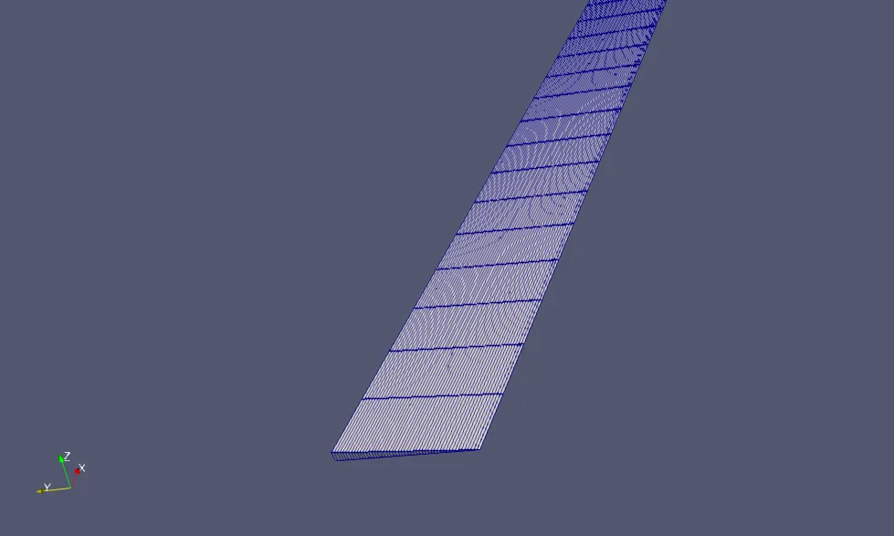
A circular pipe of 0.02m dia and 2.5m length takes a lot of computational effort and time to simulate. So, a sector of pipe which is axi symmetric is considered for simulation.
Radius of the sector will be 0.01m and angle is considered as 4°.
To create geometry and to mesh, a MATLAB function is written to generate blockMeshDict file.
Inputs to the function are
Reynolds no. = 2100
diameter = 20mm
angle(theta) = 4°
no. of cells in local X direction = 50
no. of cells in local Y direction = 1
no. of cells in local Z direction = 500
Grading along all axes is considered to be 1.
% file parsing
% creating blockmeshdict file of openfoam

function [l_t,v0,v1,v2,v3,v4,v5] = blockMeshDict(re,d,theta,nx,ny,nz,g1,g2,g3)

r = d/2;
l_e = 0.05*re*d;
l_t = l_e + 400;

v0 = [0 0 0];
v1 = [0 r*cosd(theta/2) -r*sind(theta/2)];
v2 = [0 r*cosd(theta/2) r*sind(theta/2)];
v3 = [l_t 0 0];
v4 = [l_t r*cosd(theta/2) -r*sind(theta/2)];
v5 = [l_t r*cosd(theta/2) r*sind(theta/2)];

f1 = fopen('blockMeshDict.txt','w');
fprintf(f1,'/*--------------------------------*- C++ -*-------------------------------------------*\n');
fprintf(f1,'  =========                |\n');
fprintf(f1,'  \\      /  F ield         | OpenFOAM: The Open Source CFD Toolbox\n');
fprintf(f1,'   \\    /   O peration     | Website:  https://openfoam.org\n');
fprintf(f1,'    \\  /    A nd           | Version:  8\n');
fprintf(f1,'     \\/     M anipulation  |\n');
fprintf(f1,'*---------------------------------------------------------------------------*/\n');
fprintf(f1,'FoamFile\n');
fprintf(f1,'{\n');
fprintf(f1,'    version     2.0;\n');
fprintf(f1,'    format      ascii;\n');
fprintf(f1,'    class       dictionary;\n');
fprintf(f1,'    object      blockMeshDict;\n');
fprintf(f1,'}\n');
fprintf(f1,'// * * * * * * * * * * * * * * * * * * * * * * * * * * * * * * * * * * * * * //\n\n');
fprintf(f1,'convertToMeters 0.001;\n\n');
fprintf(f1,'vertices\n');
fprintf(f1,'(\n');
fprintf(f1,'    (');
fprintf(f1,'%d %d %d)\n',v0(1),v0(2),v0(3));
fprintf(f1,'    (');
fprintf(f1,'%1.3f %1.3f %1.3f)\n',v1(1),v1(2),v1(3));
fprintf(f1,'    (');
fprintf(f1,'%1.3f %1.3f %1.3f)\n',v2(1),v2(2),v2(3));
fprintf(f1,'    (');
fprintf(f1,'%1.3f %1.3f %1.3f)\n',v3(1),v3(2),v3(3));
fprintf(f1,'    (');
fprintf(f1,'%1.3f %1.3f %1.3f)\n',v4(1),v4(2),v4(3));
fprintf(f1,'    (');
fprintf(f1,'%1.3f %1.3f %1.3f)\n',v5(1),v5(2),v5(3));
fprintf(f1,');\n\n');
fprintf(f1,'blocks\n');
fprintf(f1,'(\n');
fprintf(f1,'    hex (0 1 2 0 3 4 5 3) (%d %d %d) simpleGrading (%1.2f %1.2f %1.2f)\n', nx,ny,nz,g1,g2,g3);
fprintf(f1,');\n\n');
fprintf(f1,'edges\n');
fprintf(f1,'(\n');
fprintf(f1,'    arc 1 2 (0 %1.2f 0)\n', r);
fprintf(f1,'    arc 4 5 (%1.2f %1.2f 0)\n', l_t,r);
fprintf(f1,');\n\n');
fprintf(f1,'boundary\n');
fprintf(f1,'(\n');
fprintf(f1,'    inlet\n');
fprintf(f1,'    {\n');
fprintf(f1,'        type patch;\n');
fprintf(f1,'        faces\n');
fprintf(f1,'        (\n');
fprintf(f1,'            (0 1 2 0)\n');
fprintf(f1,'        );\n');
fprintf(f1,'    }\n\n');
fprintf(f1,'    outlet\n');
fprintf(f1,'    {\n');
fprintf(f1,'        type patch;\n');
fprintf(f1,'        faces\n');
fprintf(f1,'        (\n');
fprintf(f1,'            (3 5 4 3)\n');
fprintf(f1,'        );\n');
fprintf(f1,'    }\n\n');
fprintf(f1,'    noSlipWall\n');
fprintf(f1,'    {\n');
fprintf(f1,'        type wall;\n');
fprintf(f1,'        faces\n');
fprintf(f1,'        (\n');
fprintf(f1,'            (1 4 5 2)\n');
fprintf(f1,'        );\n');
fprintf(f1,'    }\n\n');
fprintf(f1,'    front\n');
fprintf(f1,'    {\n');
fprintf(f1,'        type wedge;\n');
fprintf(f1,'        faces\n');
fprintf(f1,'        (\n');
fprintf(f1,'            (0 3 4 1)\n');
fprintf(f1,'        );\n');
fprintf(f1,'    }\n\n');
fprintf(f1,'    back\n');
fprintf(f1,'    {\n');
fprintf(f1,'        type wedge;\n');
fprintf(f1,'        faces\n');
fprintf(f1,'        (\n');
fprintf(f1,'            (0 2 5 3)\n');
fprintf(f1,'        );\n');
fprintf(f1,'    }\n');
fprintf(f1,');\n\n');
fprintf(f1,'mergePatchPairs\n');
fprintf(f1,'(\n');
fprintf(f1,');\n\n');
fprintf(f1,'// ************************************************************************* //');
After generating blockMeshDict file, boundary conditions and transport properties must be specified.
Water is condisered as the flow fluid. As stated above, reynolds number is considered 2100.
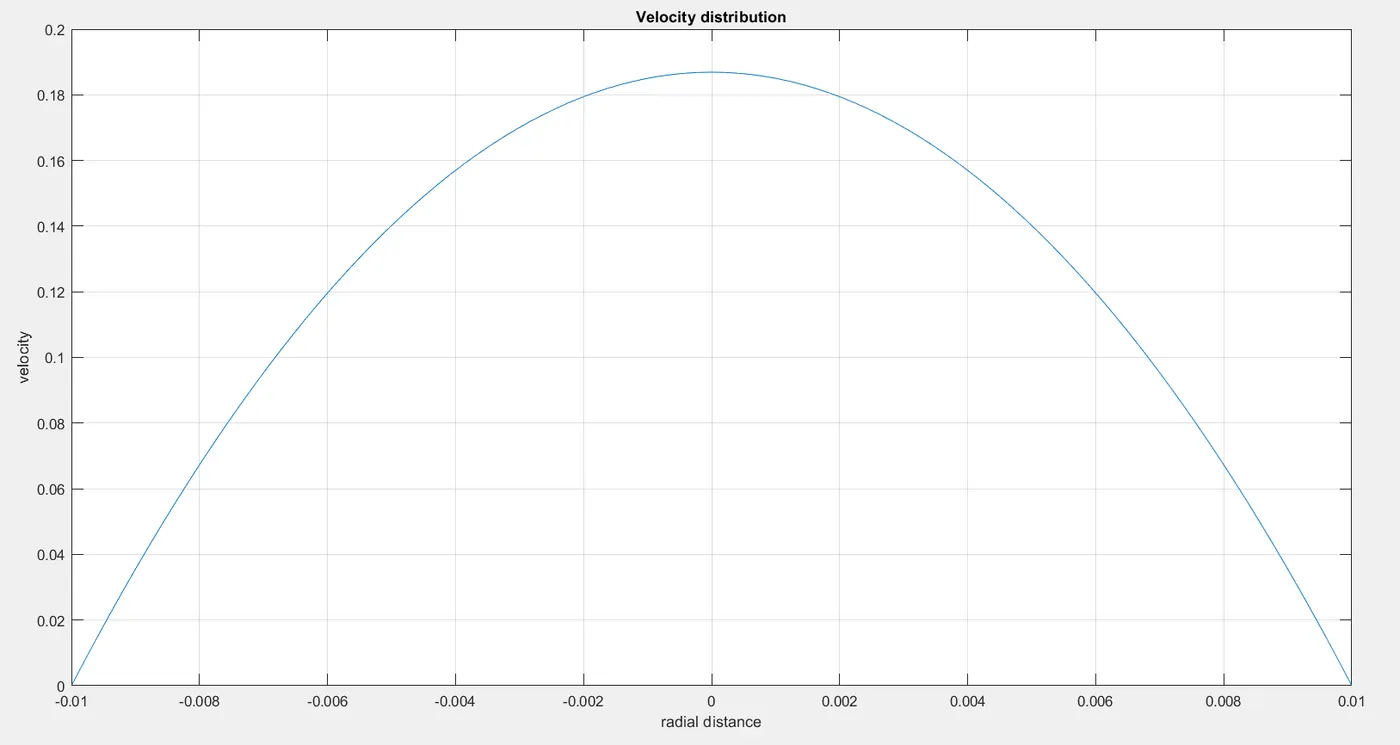
A MATLAB code is written to find the input velocity and pressure. Also, velocity profile is generated based on Hagen Poiseuille's equation.
% calculating velocity

clear all
close all
clc

re = 2100;
rho = 1000;
d = 0.02;
r = d/2;
mu = 8.9e-4;
nu = mu/rho;
c = 0.5;
nx = 500;
ny = 50;

% hydrodynamic entrance length for laminar flow
l_e = 0.05*re*d;
l_t = l_e + 0.4;

dx = l_t/(nx-1);
dy = r/(ny-1);

% re = (rho*va*d)/mu

vavg = (re*mu)/(rho*d);

vmax = 2*vavg;

dp_s = (8*mu*0.4*vavg)/r^2;

dp_k = dp_s/rho;

dt = (c*dx)/vavg;

ry = zeros(1,100);

ry(1) = -0.01;

for i = 2:(2*ny)

    ry(i) = ry(i-1)+dy;

end

for j = 1:(2*ny)

    v(j) = vmax*(1-((ry(j))^2/r^2));

end

plot(ry,v);
grid on;
axis([-0.01 0.01 0 0.2]);
xlabel('radial distance');
ylabel('velocity');
title('Velocity distribution');
Reynolds number, `Re = (rho*v_(avg)*d)/mu`--> (2)
where mu is dynamic viscosity (8.9e-4 Pa.s) and rho is density (1000 kg/m^3).
From this, the average velocity is calculated and given as input velocity.
Based on Hagen Poiseuielle's equation,
`v_(max) = 2*v_(avg)`
`v = v_(max)*(1-r^2/R^2)` --> (3)
`pressure drop, dp_s = (8*mu*0.4*v_(avg))/R^2` --> (4)
`kinematic pressure drop, dp_k = (dp_s)/rho` --> (5)
where r is the radial distance from centre, R is the radius of pipe.
Also, courant number for non linear equation is taken as 0.5.
`Time step size, dt = (c*dx)/v_(avg)`--> (6)
From the above equations, average velocity, kinematic pressure, kinematic viscosity and time step size are obtained and provided as input.
Boundary conditions:
Velocity:
/*--------------------------------*- C++ -*----------------------------------*\
  =========                 |
  \\      /  F ield         | OpenFOAM: The Open Source CFD Toolbox
   \\    /   O peration     | Website:  https://openfoam.org
    \\  /    A nd           | Version:  8
     \\/     M anipulation  |
\*---------------------------------------------------------------------------*/
FoamFile
{
    version     2.0;
    format      ascii;
    class       volVectorField;
    object      U;
}
// * * * * * * * * * * * * * * * * * * * * * * * * * * * * * * * * * * * * * //

dimensions      [0 1 -1 0 0 0 0];

internalField   uniform (0 0 0);

boundaryField
{
    inlet
    {
        type            fixedValue;
        value           uniform (0.0935 0 0);
    }

    outlet
    {
        type            zeroGradient;
    }

    noSlipWall
    {
        type            noSlip;
    }

    front
    {
        type            wedge;
    }

    back
    {
        type            wedge;
    }
}

// ************************************************************************* //
Pressure:
/*--------------------------------*- C++ -*----------------------------------*\
  =========                 |
  \\      /  F ield         | OpenFOAM: The Open Source CFD Toolbox
   \\    /   O peration     | Website:  https://openfoam.org
    \\  /    A nd           | Version:  8
     \\/     M anipulation  |
\*---------------------------------------------------------------------------*/
FoamFile
{
    version     2.0;
    format      ascii;
    class       volScalarField;
    object      p;
}
// * * * * * * * * * * * * * * * * * * * * * * * * * * * * * * * * * * * * * //

dimensions      [0 2 -2 0 0 0 0];

internalField   uniform 0;

boundaryField
{
    inlet
    {
        type            zeroGradient;
    }

    outlet
    {
        type            fixedValue;
        value           uniform 0.00027;
    }

    noSlipWall
    {
        type            zeroGradient;
    }

    front
    {
        type            wedge;
    }

    back
    {
        type            wedge;
    }
}

// ************************************************************************* //
Transport Properties:
/*--------------------------------*- C++ -*----------------------------------*\
  =========                 |
  \\      /  F ield         | OpenFOAM: The Open Source CFD Toolbox
   \\    /   O peration     | Website:  https://openfoam.org
    \\  /    A nd           | Version:  8
     \\/     M anipulation  |
\*---------------------------------------------------------------------------*/
FoamFile
{
    version     2.0;
    format      ascii;
    class       dictionary;
    location    "constant";
    object      transportProperties;
}
// * * * * * * * * * * * * * * * * * * * * * * * * * * * * * * * * * * * * * //

nu              [0 2 -1 0 0 0 0] 8.9e-7;


// ************************************************************************* //
Control Dict:
/*--------------------------------*- C++ -*----------------------------------*\
  =========                 |
  \\      /  F ield         | OpenFOAM: The Open Source CFD Toolbox
   \\    /   O peration     | Website:  https://openfoam.org
    \\  /    A nd           | Version:  8
     \\/     M anipulation  |
\*---------------------------------------------------------------------------*/
FoamFile
{
    version     2.0;
    format      ascii;
    class       dictionary;
    location    "system";
    object      controlDict;
}
// * * * * * * * * * * * * * * * * * * * * * * * * * * * * * * * * * * * * * //

application     icoFoam;

startFrom       startTime;

startTime       0;

stopAt          endTime;

endTime         21.44;

deltaT          0.0268;

writeControl    timeStep;

writeInterval   20;

purgeWrite      0;

writeFormat     ascii;

writePrecision  6;

writeCompression off;

timeFormat      general;

timePrecision   6;

runTimeModifiable true;


// ************************************************************************* //
Outputs:
1. BlockMeshDict file generated by MATLAB code:
/*--------------------------------*- C++ -*-------------------------------------------*
  =========                |
  \      /  F ield         | OpenFOAM: The Open Source CFD Toolbox
   \    /   O peration     | Website:  https://openfoam.org
    \  /    A nd           | Version:  8
     \/     M anipulation  |
*---------------------------------------------------------------------------*/
FoamFile
{
    version     2.0;
    format      ascii;
    class       dictionary;
    object      blockMeshDict;
}
// * * * * * * * * * * * * * * * * * * * * * * * * * * * * * * * * * * * * * //

convertToMeters 0.001;

vertices
(
    (0 0 0)
    (0.000 9.994 -0.349)
    (0.000 9.994 0.349)
    (2500.000 0.000 0.000)
    (2500.000 9.994 -0.349)
    (2500.000 9.994 0.349)
);

blocks
(
    hex (0 1 2 0 3 4 5 3) (50 1 500) simpleGrading (1.00 1.00 1.00)
);

edges
(
    arc 1 2 (0 10.00 0)
    arc 4 5 (2500.00 10.00 0)
);

boundary
(
    inlet
    {
        type patch;
        faces
        (
            (0 1 2 0)
        );
    }

    outlet
    {
        type patch;
        faces
        (
            (3 5 4 3)
        );
    }

    noSlipWall
    {
        type wall;
        faces
        (
            (1 4 5 2)
        );
    }

    front
    {
        type wedge;
        faces
        (
            (0 3 4 1)
        );
    }

    back
    {
        type wedge;
        faces
        (
            (0 2 5 3)
        );
    }
);

mergePatchPairs
(
);

// ************************************************************************* //
Geometry & Mesh:
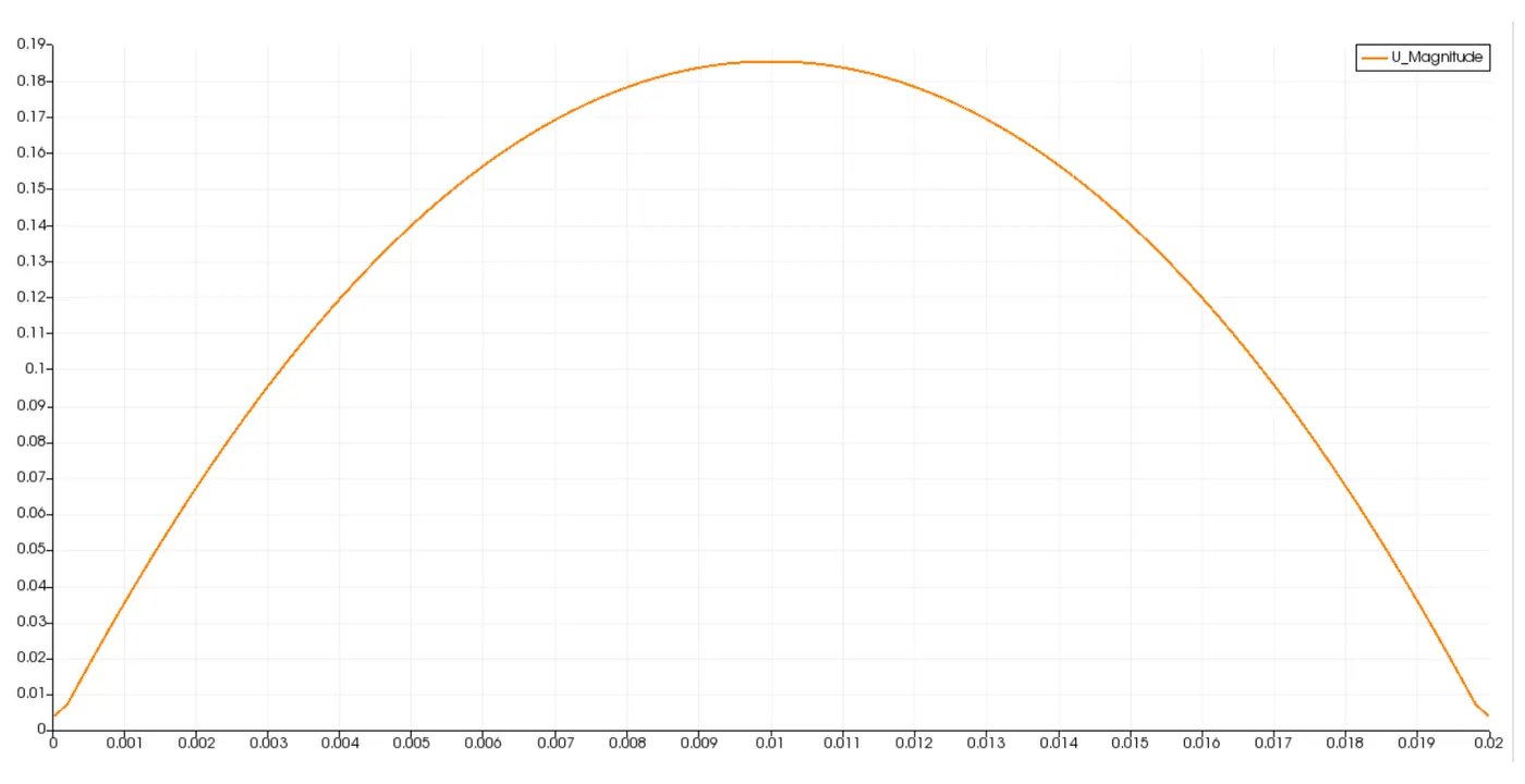
2. Velocity distribution at partcular cross-sections at various distances from inlet of pipe simulated using Openfoam:
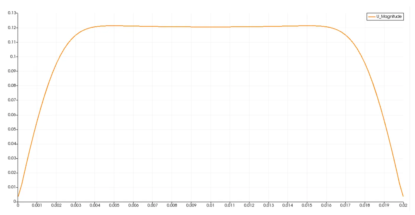
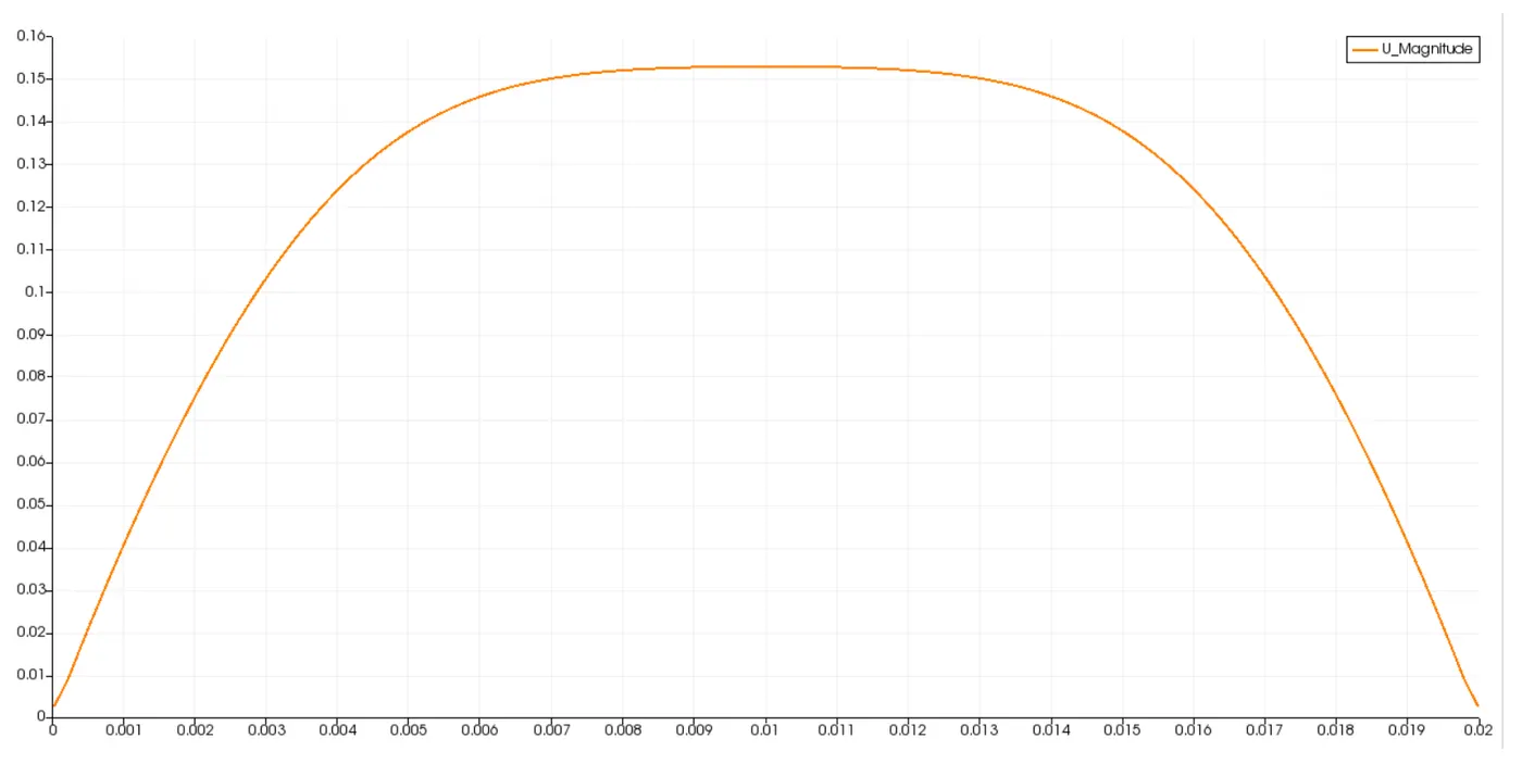
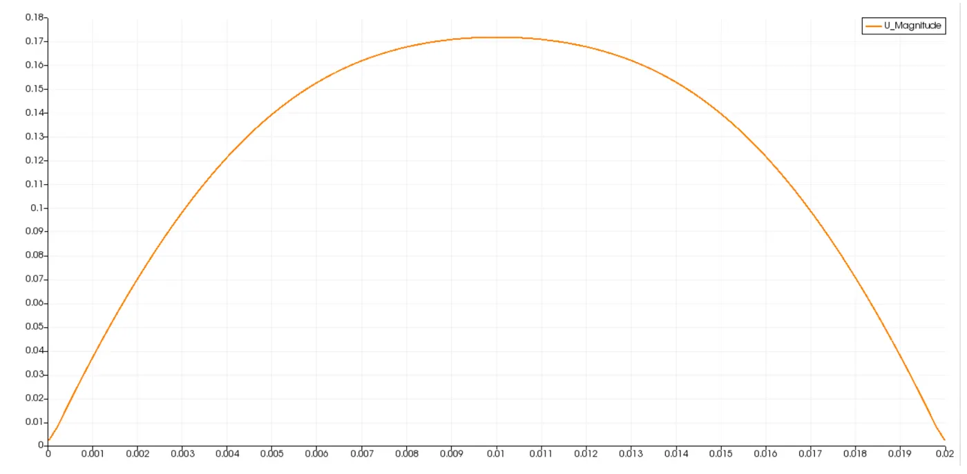
Graphs are plotted to find out the velocity distribution with diameter of pipe.
X - axis : Diameter of pipe with center at 0.01m.
Y - axis : Velocity
(i) At 0.1m distance from inlet:
(ii) At 0.5m distance from inlet:
(iii) At 1.0m distance from inlet:
(iv) At 1.5m distance from inlet:
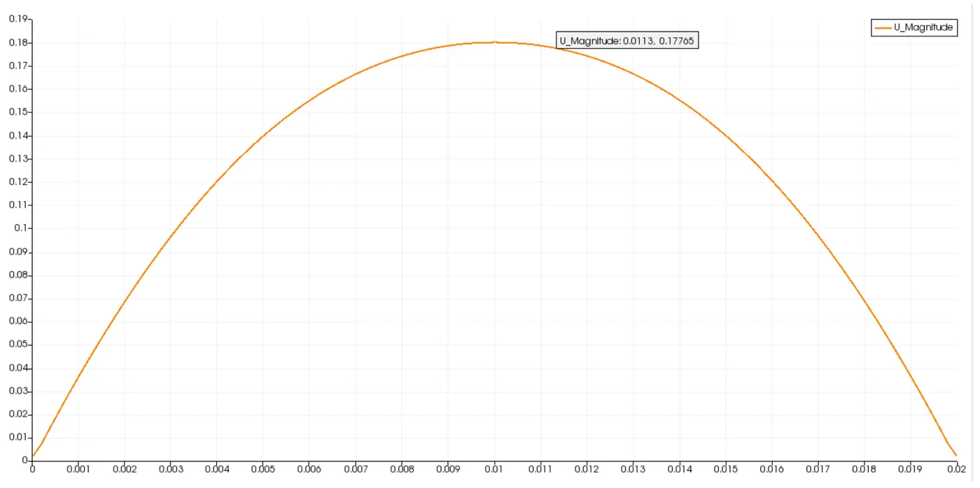
(v) At 2.0m distance from inlet:
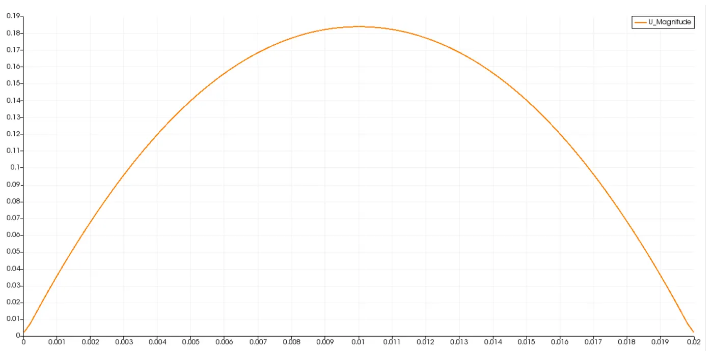
(vi) At 2.1m distance from inlet:
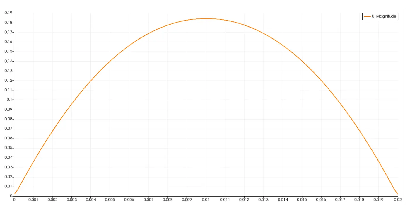
(vii) At 2.3m distance from inlet: (Fully Developed Flow)
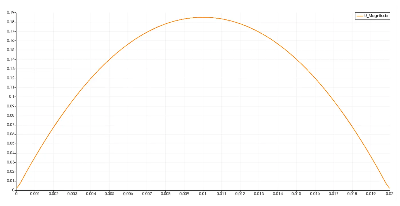
(viii) At 2.5m distance from inlet: (Fully Developed Flow)
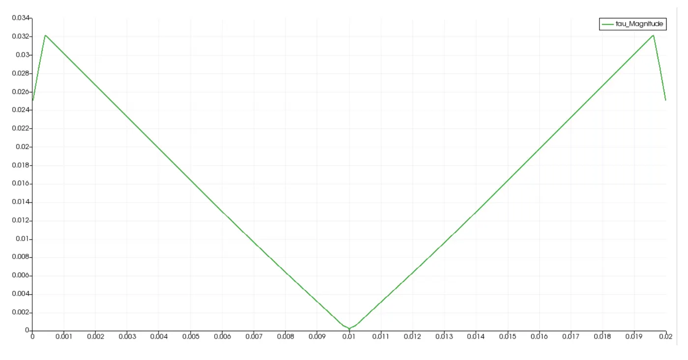
3. Shear stress in the pipe during fully developed flow (2.4m distance from inlet):
3. Validation - velocity distribution during fully developed flow obtained using Hagen Poiseuille's equation from MATLAB:
Conclusions:
1. From the above plots, it is observed that velocity distribution keeps changing till 2.1m distance from inlet. After 2.1m, velocity distribution is uniform throughout the remaining length. A fully developed flow after 2.1m is observed.
This is validated with equation (1) by which the fully developed flow for a pipe of diameter 0.02m and with reynolds number 2100 is obtained after 2.1m.
Also, the velocity distribution at fully developed flow is found to be parabolic with maximum velocity (approx. 0.185 m/sec) at centre of the pipe. This is validated by Hagen Poiseuille equation solved in MATLAB and the obtained velocity distribution and max. velocity are same as obtained in openfoam (Figure 3).
2. Shear stress distribution for fully developed flow is found out and is observed that the max. shear stress is near the wall and the minimum is at the centre. This is because the wall acts as a resistnace to fluid flow, shear force acts on the fluid layers near the walls thereby inducing shear stress. Further down from the wall, shear forces are not as high as near the wall and is almost zero at the centre. As the flow is laminar, the fluid layers move parallel to each other and least resistance is at the centre which makes the shear stress to be almost zero.
As the shear stress is least at the centre, the fluid moves with maximum velocity at the centre.