Week 3 - Taylor table method and Matlab code
Derivation for fourth order approximation of second order derivative:
1. Central Differencing scheme:
In this scheme, the node(point) at which the second order derivative should be calculated is placed at the centre while the remaining nodes are to the left and right.
No. of nodes = (order of derivative + order of approximation -1)
= 2 + 4-1
= 5.
So, five nodes should be taken to calcuate the second order deriuvative with fourthj order approximation.
let those points be (i-2), (i-1), i, (i+1), (i+2)
let the distance between each points be dx.
let (dx^(2))*(d^f/dx^2) = a*f(i-2) + b*f(i-1) + c*f(i) + d*f(i+1) e*f(1+2) --->(1)
Also, let df/dx = f', d^f/dx^2=f'', d^3f/dx^3=f''', d^4f/dx^4=f'''', d^5f/dx^5 =f'''''
Using taylor series expansion,
a*f(1-2) = a*[f(i) - f'(i)(2*dx)/1! + f''(i)(2*dx)^2/2! - f'''(i)(2*dx)^3/3! + f''''(i)(2*dx)^4/4! - f'''''(i)(2*dx)^5/5! + ...]
b*f(i-1) = b*[f(i) - f'(i)(dx)/1! + f''(i)(dx)^2/2! - f'''(i)(dx)^3/3! + f''''(i)(dx)^4/4! - f'''''(i)(dx)^5/5! + ...]
c*f(i) = c*f(i)
d*f(i+1) = d*[f(i) + f'(i)(dx)/1! + f''(i)(dx)^2/2! + f'''(i)(dx)^3/3! + f''''(i)(dx)^4/4! + f'''''(i)(dx)^5/5! + ...]
e*f(i+2) = e*[f(i) + f'(i)(2*dx)/1! + f''(i)(2*dx)^2/2! + f'''(i)(2*dx)^3/3! + f''''(i)(2*dx)^4/4! + f'''''(i)(2*dx)^5/5! + ...]
Taylor table:
A table showing the coefficients for all ith teems and their derivatives
| f(i) | dx*f'(i) | dx^2*f''(i) | dx^3*f'''(i) | dx^4*f''''(i) | dx^5*f'''''(i) | |
| f(i-2) | a | -2a | 4a/2 | -8a/6 | 16a/24 | -32a/120 |
| f(i-1) | b | -b | b/2 | -b/6 | b/24 | -b/120 |
| f(i) | c | 0 | 0 | 0 | 0 | 0 |
| f(i+1) | d | d | d/2 | d/6 | d/24 | d/120 |
| f(i+2) | e | 2e | 4e/2 | 8e/6 | 16e/24 | 32e/120 |
| dx^2*f''(x) | 0 | 0 | 1 | 0 | 0 |
For finding second order derivative, only the terms having the coefficient as f'' should be 1, remaining terms will be zero.
taking the sum of terms for each derivative,
a+b+c+d+e = 0
-2a-2b+d+2e=0
4a/2+b/2+d/2+4e/2=1
-8a/6-b/6+d/6+8e/6=0
16a/24+b/24+d/24+16e/24=0
Arranging them in matrix form,
[1 1 1 1 1; -2 -1 0 1 2; 4/2 1/2 0 1/2 4/2; -8/6 -1/6 0 1/6 8/6; 16/24 1/24 0 1/24 16/24]*[a;b;c;d;e] = [0;0;1;0;0]
Solving the above matrix using mtarix inversion method in MATLAB, we get the values for a,b,c,d,e as
a=-0.0833; b=1.3333; c=-2.5; d=1.3333; e=-0.08333
Subsittuting these values in eq. (1) we get
f''(x) = [-0.0833f(i-2) + 1.3333f(i-1) -2.5f(i) +1.3333f(i+1) - 0.08333f(i+2)]/(dx^2)
2. Skewed right side scheme:
In this scheme, the node(point) at which the second order derivative should be calculated is the first point while the remaining nodes are to the right.
No. of nodes = (order of derivative + order of approximation
= 2 + 4
= 6
So, six nodes should be taken to calcuate the second order deriuvative with fourth order approximation.
let those points be i, (i+1), (i+2), (i+3), (i+4), (i+5)
let the distance between each points be dx.
let (dx^(2))*(d^f/dx^2) = a*f(i) + b*f(i+1) + c*f(i+2) + d*f(i+3)+ e*f(1+4) + g*f(i+5) --->(2)
a*f(i) = a*f(i)
b*f(i+1) = b*[f(i) + f'(i)(dx)/1! + f''(i)(dx)^2/2! + f'''(i)(dx)^3/3! + f''''(i)(dx)^4/4! + f'''''(i)(dx)^5/5! + f''''''(i)(dx)^6/6!...]
c*f(i+2) = c*[f(i) + f'(i)(2*dx)/1! + f''(i)(2*dx)^2/2! + f'''(i)(2*dx)^3/3! + f''''(i)(2*dx)^4/4! + f'''''(i)(2*dx)^5/5! +f''''''(i)(2*dx)^6/6! ...]
d*f(i+3) = d*[f(i) + f'(i)(3*dx)/1! + f''(i)(3*dx)^2/2! + f'''(i)(3*dx)^3/3! + f''''(i)(3*dx)^4/4! + f'''''(i)(3*dx)^5/5! +f''''''(i)(3*dx)^6/6! ...]
e*f(i+4) = e*[f(i) + f'(i)(4*dx)/1! + f''(i)(4*dx)^2/2! + f'''(i)(4*dx)^3/3! + f''''(i)(4*dx)^4/4! + f'''''(i)(4*dx)^5/5! +f''''''(i)(4*dx)^6/6! ...]
g*f(i+5) = g*[f(i) + f'(i)(5*dx)/1! + f''(i)(5*dx)^2/2! + f'''(i)(5*dx)^3/3! + f''''(i)(5*dx)^4/4! + f'''''(i)(5*dx)^5/5! +f''''''(i)(5*dx)^6/6! ...]
Taylor table:
A table showing the coefficients for all ith teems and their derivatives
| f(i) | dx*f'(i) | dx^2*f''(i) | dx^3*f'''(i) | dx^4*f''''(i) | dx^5*f'''''(i) | dx^6*f''''''(x) | |
| f(i) | a | 0 | 0 | 0 | 0 | 0 | 0 |
| f(i+1) | b | b | b/2 | b/6 | b/24 | b/120 | b/720 |
| f(i+2) | c | 2c | 4c/2 | 8c/6 | 16c/24 | 32c/120 | 64c/720 |
| f(i+3) | d | 3d | 9d/2 | 27d/6 | 81d/24 | 243d/120 | 729d/720 |
| f(i+4) | e | 4e | 16e/2 | 64e/6 | 256e/24 | 1024e/120 | 4096e/720 |
| f(i+5) | g | 5g | 25g/2 | 125g/6 | 625g/24 | 3125g/120 | 15625g/720 |
| dx^2*f''(x) | 0 | 0 | 1 | 0 | 0 | 0 |
For finding second order derivative, only the terms having the coefficient as f'' should be 1, remaining terms will be zero.
taking the sum of terms for each derivative,
a+b+c+d+e+g = 0
b+2c+3d+4e+5g=0
b/2+4c/2+9d/2+16e/2+25g/2=1
b/6+8c/6+27d/6+64e/6+125g/6=0
b/24+16c/24+81d/24+256e/24+625g/24=0
b/120+32c/120+243d/120+1024e/120+3125g/120=0
Arranging them in matrix form,
[1 1 1 1 1 1; 0 1 2 3 4 5; 0 1/2 4/2 9/2 16/2 25/2; 0 1/6 8/6 27/6 64/6 125/6; 0 1/24 16/24 81/24 256/24 625/24; 0 1/120 32/120 243/120 1024/120 3125/120]*[a;b;c;d;e;g] = [0;0;1;0;0;0]
Solving the above matrix using mtarix inversion method in MATLAB, we get the values for a,b,c,d,e,g as
a=3.75; b=-12.8333; c=-17.8333; d=-13; e=5.0833, g=-0.8333
Subsittuting these values in eq. (2) we get
f''(x) = [3.75f(i) - 12.8333f(i+1) + 17.8333f(i+2) -13f(i+3) + 5.08333f(i+4) - 0.8333f(i+5)]/(dx^2)
Also,
f''(x) = (a+b+c+d+e+g )f(i) + (b+2c+3d+4e+5g)dx*f'(i) + (b/2+4c/2+9d/2+16e/2+25g/2)dx^2*f''(i) + (b/6+8c/6+27d/6+64e/6+125g/6)dx^3*f'''(i) + (b/24+16c/24+81d/24+256e/24+625g/24)dx^4f''''(i) + (b/120+32c/120+243d/120+1024e/120+3125g/120)dx^5f'''''(i) + (b/720+64e/720+729d/720+4096d/720+15625g/720)dx^6*f''''''(i)
we know that terms of f(i), f'(i), f'''(i), f''''(i) and f'''''(i) are zero and f''(i) will be 1.
then,
f''(x) = (b/2+4c/2+9d/2+16e/2+25g/2)dx^2*f''(i) + (b/720+64e/720+729d/720+4096d/720+15625g/720)dx^6*f''''''(i)
Duviding with dx^2
f''(x) = (b/2+4c/2+9d/2+16e/2+25g/2)f''(i) + O(dx^4)
If we neglect the dx^ terms, the above approximatio wil be of order 4.
Hence it is proved that the skewed right scheme is of order 4.
3. Skewed left side scheme:
In this scheme, the node(point) at which the second order derivative should be calculated is the last point while the remaining nodes are to the left.
No. of nodes = (order of derivative + order of approximation)
= 2 + 4
= 6
So, six nodes should be taken to calcuate the second order deriuvative with fourth order approximation.
let those points be (i-5), (i-4), (i-3), (i-2), (i-1),i
let the distance between each points be dx.
let (dx^(2))*(d^f/dx^2) = a*f(i-5) + b*f(i-4) + c*f(i-3) + d*f(i-2)+ e*f(1-1) + g*f(i) --->(3)
g*f(i) = g*f(i)
e*f(i-1) = e*[f(i) - f'(i)(dx)/1! + f''(i)(dx)^2/2! - f'''(i)(dx)^3/3! + f''''(i)(dx)^4/4! - f'''''(i)(dx)^5/5! + f''''''(i)(dx)^6/6!...]
d*f(i-2) = d*[f(i) - f'(i)(2*dx)/1! + f''(i)(2*dx)^2/2! - f'''(i)(2*dx)^3/3! + f''''(i)(2*dx)^4/4! - f'''''(i)(2*dx)^5/5! +f''''''(i)(2*dx)^6/6! ...]
c*f(i-3) = c*[f(i) - f'(i)(3*dx)/1! + f''(i)(3*dx)^2/2! - f'''(i)(3*dx)^3/3! + f''''(i)(3*dx)^4/4! - f'''''(i)(3*dx)^5/5! +f''''''(i)(3*dx)^6/6! ...]
b*f(i-4) = b*[f(i) - f'(i)(4*dx)/1! + f''(i)(4*dx)^2/2! - f'''(i)(4*dx)^3/3! + f''''(i)(4*dx)^4/4! - f'''''(i)(4*dx)^5/5! +f''''''(i)(4*dx)^6/6! ...]
a*f(i-5) = a*[f(i) - f'(i)(5*dx)/1! + f''(i)(5*dx)^2/2! - f'''(i)(5*dx)^3/3! + f''''(i)(5*dx)^4/4! - f'''''(i)(5*dx)^5/5! +f''''''(i)(5*dx)^6/6! ...]
Taylor table:
A table showing the coefficients for all ith teems and their derivatives
| f(i) | dx*f'(i) | dx^2*f''(i) | dx^3*f'''(i) | dx^4*f''''(i) | dx^5*f'''''(i) | |
| f(i-5) | a | -5a | 25a/2 | -125a/6 | 625a/24 | -3125a/120 |
| f(i-4) | b | -4b | 16b/2 | -64b/6 | 256b/24 | -1024b/120 |
| f(i-3) | c | -3c | 9c/2 | -27c/6 | 81c/24 | -243c/120 |
| f(i-2) | d | -2d | 4d/2 | -8d/6 | 16d/24 | 32d/120 |
| f(i-1) | e | -e | e/2 | -e/6 | e/24 | -e/120 |
| f(i) | g | 0 | 0 | 0 | 0 | 0 |
| dx^2*f''(x) | 0 | 0 | 1 | 0 | 0 | 0 |
For finding second order derivative, only the terms having the coefficient as f'' should be 1, remaining terms will be zero.
taking the sum of terms for each derivative,
a+b+c+d+e+g = 0
-5a-4b-3c-2d-e=0
25a/2+16b/2+9c/2+4d/2+e/2=1
-125a/6-64b/6-27c/6-8d/6-e/6=0
625a/24+256b/24+81c/24+16d/24+e/24=0
-3125a/120-1024b/120-243c/120-32d/120-e/120 = 0
Arranging them in matrix form,
[1 1 1 1 1 1; -5 -4 -3 -2 -1 0; 25/2 16/2 9/2 4/2 1/2 0; -125/6 -64/6 -27/6 -8/6 -1/9 0; 625/24 256/24 81/24 16/24 1/24 0; -3125/120 -1024/120 -243/120 -32/120 -1/120 0]
Solving the above matrix using mtarix inversion method in MATLAB, we get the values for a,b,c,d,e,g as
g=3.75; e=-12.8333; d=-17.8333; c=-13; b=5.0833, a=-0.8333
Subsittuting these values in eq. (2) we get
f''(x) = [3.75f(i) - 12.8333f(i-1) + 17.8333f(i-2) -13f(i-3) + 5.08333f(i-4) - 0.8333f(i-5)]/(dx^2)
MATLAB Code:
A code is written in MATLAB to find the error for these above numerical approximations at different values of dx.
For this purpsoe , analtyical solution should be calculated and should be compared with numerical approximations.
given function is exp(x)*cos(x)
Its derivative anlatyically is d[f(x)*g(x)] = f(x)*d[g(x)] + g(x)*d[f(x)]
so, derivative of given function is exp(x)*(cosx - sinx).
% fourth order approximations for second order derivative
% given function is e^x*cos(x)

clear all
close all
clc

x=pi/3;
dx=linspace(10^(-2),10^(-1),10);

for i = 1:length(dx)

%forward differencing scheme
% [(3.75*f(x)) - (12.8333*f(x+dx(i))) + (17.8333*f(x+(2*dx(i)))) -
% (13*f(x+(3*dx(i)))) +(5.08333*f(x+(4*dx(i)))) - (0.8333*f(x+(5*dx(i))))]/(dx(i)^(2))

forward_difference(i) = ((3.75*((exp(x))*cos(x))) - (12.8333*((exp(x+dx(i)))*cos(x+dx(i))))...
    +(17.8333*((exp(x+(2*dx(i))))*cos(x+(2*dx(i))))) - (13*((exp(x+(3*dx(i))))*cos(x+(3*dx(i)))))...
    + (5.08333*((exp(x+(4*dx(i))))*cos(x+(4*dx(i))))) - ...
    (0.8333*((exp(x+(5*dx(i))))*cos(x+(5*dx(i))))))/(dx(i)^(2))

%backward differencing scheme
% [(3.75*f(x)) - (12.8333*f(x-dx(i))) + (17.8333*f(x-(2*dx(i)))) -
% (13*f(x-(3*dx(i)))) +(5.08333*f(x-(4*dx(i)))) - (0.8333*f(x-(5*dx(i))))]/(dx(i)^(2))

backward_difference(i) = ((3.75*((exp(x))*cos(x))) - (12.8333*((exp(x-dx(i)))*cos(x-dx(i))))...
    +(17.8333*((exp(x-(2*dx(i))))*cos(x-(2*dx(i))))) - (13*((exp(x-(3*dx(i))))*cos(x-(3*dx(i)))))...
    + (5.08333*((exp(x-(4*dx(i))))*cos(x-(4*dx(i))))) - ...
    (0.8333*((exp(x-(5*dx(i))))*cos(x-(5*dx(i))))))/(dx(i)^(2))

%central differencing scheme
%[-(0.0.8333*f(x-(2*dx(i)))) + (1.8333*f(x-dx(i))) - (2.5*f(x)) + (1.3333*f(x+dx(i)))
% - (0.08333*f(x+(2*dx(i))))]/(dx(i)^(2))

central_difference(i) = (-(0.08333*((exp(x-(2*dx(i))))*cos(x-(2*dx(i))))) + ...
    (1.3333*((exp(x-dx(i)))*cos(x-dx(i)))) - (2.5*((exp(x))*cos(x))) +...
    (1.3333*((exp(x+dx(i)))*cos(x+dx(i)))) - ...
    (0.08333*((exp(x+(2*dx(i))))*cos(x+(2*dx(i))))))/(dx(i)^(2))

analytical_value  = exp(x)*(cos(x)-sin(x))

error_forward(i) = abs(forward_difference(i) - analytical_value)

error_backward(i) = abs(backward_difference(i) - analytical_value)

error_central(i) = abs(central_difference(i) - analytical_value)

end

aa = plot(dx,error_forward);
hold on
bb = plot(dx,error_backward);
cc = plot(dx,error_central);

legend([aa,bb,cc],'skewed right','skewed left','central difference');
xlabel('dx');
ylabel('error');
let us calculate derivative at x = pi/3 and the range of dx will be linspace(10^-2,10^-1,10)
linspace will assign 10 values in between 10^-2 and 10^-1 in matrix dx.
A for loop from i = to lenghe(dx) is introduced as we need to calculate error for multiple dx values.
length(dx) is the no. of elements in dx matrix which is 10.
So, for i = 1: 10,
next all the equations which are derived above are written
dx value in the equations should be dx(i).
This is because, initiallt the i value will be 1 and dx(i) will be dx(1). dx(1) accesses thte first element in matrix dx and performs calculations. This i value keeps on incresing until it reaches i=10.
Values for skewed right are stored in matrix "forward_difference".
values for skewed left are stored in "backward_difference".
values for centra;l difference are stored in "central_difference"
error is the difference between numeriacl value and analytival value.
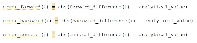
These errors are stored in their respective error matrices.
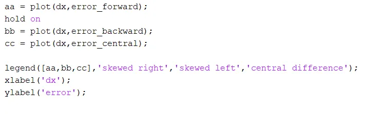
A plot is drawn with dx values on x axis and error values on Y axis.
Outputs:
A plot showing variation of error with dx values for 3 numerical approximations is shown
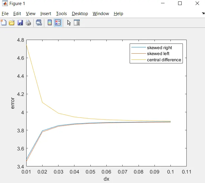
From the baove plot, it can be observed that the error value for
(skewed left)<(skewed right)<(central difference).
Therefore, skewed schemes are preferbale to use as they produce less error.
This is because, consider a fluid is flowing from left to right.
If skewed left method is used instead of central difference, the skewed left method takes information from 5 nodes behind whereas the central scheme takes the information from only 2 nodes behind.
This lead to lesser error in skewed left method.